This is one of the most common constructions. The rate of change of the state variable is a function of its present value.

 

Loading time-series data into a simple variable parameter is described in the Simile Help file.  

Sometimes, however, you may want to load a time-series for a variable parameter which is inside a multiple-instance submodel (fixed number of instances).  You want each instance to have a different time-series.

A variable parameter inside a multiple-instance submodel will want a 2-D array of values, with the outer dimension being time. You can load a 2D array directly from a .csv file using 'Data in grid', but the row numbers are the outer indices, which is the other way round from what you say you want. So: open the data file with a spreadsheet, and transpose it, save the result, then load it using the 'Data in grid' option..

Sometimes, the usual mathematical expressions aren’t enough. For example, although it’s easy to say that one variable is proportional to another, by multiplying it by a constant, it’s much harder to say that the value of a variable depends on whether another variable is above or below a threshold value. Simile’s equation language provides if...then statements as a way of handling these either / or situations. Using these conditional statements, alternative expressions are used depending on the result of evaluating a condition. For example, the overflow of water from a tank will be high if the tank is full, and zero otherwise.

Conditional statements are made up of several parts, some of which (the middle elseif parts) are optional. The general form is:

if C1 then E1 elseif C2 then E2 ..... else En

where:

• C1, C2,... are some conditions
• E1 is the expression used if the first condition is true
• E2 is the expression used if the second condition is true and the first is not
• En is the expression used if all the conditions are false

For example, if the maximum volume of the tank is stored in a variable called “Maximum”, and the amount of water in the tank is stored in a variable called “Amount” then the following expression could be used to calculate the overflow rate: “if Amount>=Maximum then 100 else 0”. In this case “Amount>=Maximum” is the condition, and 100 is the expression when the condition is true (the tank is full) and 0 is the expression when the condition is false (the tank is less than full).

Notes:

• The elseif part is optional, and you can have as many of them as you like.
• You must have the final else part.
• Each condition has three parts: any expression, a comparison operator (<, >, =), and any expression.

At heart, many Systems Dynamics models consist of differential equations, each one represented by a compartment / flow structure, though you don’t need to know this to set up the model. On the other hand, if you’re given the differential equations, it is very straightforward to enter these into the model.

For example, given the differential equation:

dx/dt = x/20 - x²/2000

you know two things:

1. there is a state variable, x, whose value changes through time; and
2. the rate of change of the value of x depends only on the value of x itself.

With this information, you can deduce that it is necessary to have one compartment, labelled “x”, one flow, labelled, say “dx by dt”, and an influence arrow from the compartment to the flow.

The equation can then be entered, exactly as given, into the equation dialgoue box for the flow. In Simile’s equation language, this is written “x/20-x^2/2000”. To run the model, and solve the differential equation, it is also necessary to know the initial value of x, i.e. the value at time zero. This is not given by the equation itself, but is usually reported, often described as the initial conditions. Enter this value in the equation bar (or equation dialogue box) for the compartment — in this example, “1” works well.

To complete this simulation, run the model for 200 time units, and display (plot) the values of the compartment and of the flow on separate graphs. Note that the value you enter for “dt” in the run control, by default “0.1”, is used as the time step for performing numerical integration by the Euler method. This particular equation is not very sensitive to the time step used, but if very rapid rates of change are encountered, it can be necessary to experiment with reducing the time step to find the optimum balance between speed of execution and numerical stability.

Note that in some mathematical notations, dx/dt is written as x with a dot above it, but the two mean exactly the same. Note also that the differential equation in this case can be broken into two parts, one positive contribution to the rate of change (an increase), x/20, and one negative contribution to the rate of change (a decrease), x²/2000. If this has a physical significance, two flows can be used, one flowing into the compartment and representing the positive contribution, and the other flowing out of the compartment and representing the negative contribution. Simile will automatically net the outflows off against the inflows in determining the overall rate of change.

Many ecological processes are influenced by several factors together. For example, plant growth may be influenced by temperature, radiation, and soil water content. It is often difficult to know how to combine the effect of these factors.

One method is to envisage each factor as having some optimum value: when all the influencing factors are at this optimum, then the process (e.g. growth) proceeds at some maximum rate. When a factor is not at its optimum value, then the rate of the process is reduced. Thus, a general solution is to use an expression of the form:

flow = flowmax*m1*m2*m3

where:

• flow is the calculated flow rate
• flowmax is the max flow rate if all influencing factors have their optimum values
• m1, m2 etc are multipliers for each influencing factor (e.g. m1 could be the temperature multiplier)

To calculate the multipliers, you might use the abs function to find out the difference between a factor and its optimum value. You then need to scale the multiplier so that it lies between zero and one. Alternatively, suppose that plants do not grow at all below Tmin nor above Tmax. Then the following expression would work:

q=(Topt-Tmin)/(Tmax-Topt),
if ((T>Tmin)&&(T<Tmax)) then
(((T-Tmin)^q) * (Tmax-T)) / (((Topt-Tmin)^q) * (Tmax-Topt))
else
0

You may notice that the above expression involves an intermediate variable q. It is a valuable feature of Simile’s equation language that expressions can often be simplified by calculating a sub-expression that is used more than once and assigning it to an intermediate variable.

The expression is also formatted to make it easier to read. The equation dialogue box preserves the formatting you enter. It doesn’t affect the parsing of the equation, but it does make it easier for the user.

It is often useful to be able to use current simulation time in your model: for example, you may want to incorporate a gradual increase in some external variable such as temperature. For this purpose, a special function called time is provided in Simile.

The time function has a value equal to the number of time units that has elapsed since the start of the simulation (which is assigned a time of zero). To help avoid any confusion, please note that it has nothing to do with the real-world time that elapses as the model runs. How long a simulation takes to run depends on how complex it is and how fast your computer is, amongst other factors, but none of these influences the time function. If you run a simulation for 100 time units, then the time function will increase from zero to 100 during the simulation. This may take 20 seconds of your time or it may take 20 minutes, depending as I say, on the model’s complexity and the speed of your computer.

You can use the time function in constructing expressions in Simile’s equation language. This gives enormous flexibility in constructing expressions. Perhaps the two most common uses are in drawing sketch graphs to illustrate how some external influence changes through time, and in constructing cycles, such as the repetition of the seasons year after year.

This is a simple example of optimizing output of a Simile model using SimileScripting and the Tcllib optimization package math::optimize. The script illustrates how to tackle this kind of problem.

"The package math::optimize is fully implemented in Tcl and no particular attention has been paid to the accuracy of the calculations. Instead, the algorithms have been used in a straightforward manner."

The script uses the procedure ::math::optimize::min_bound_1d that miminizes a function of one variable in the given interval. The procedure uses Brent's method of parabolic interpolation, protected by golden-section subdivisions if the interpolation is not converging. No guarantee is made that a global minimum is found. In the script the proceedure func is defined for ::math::optimize::min_bound_1d to evaluate. Proc func wraps up some SimileScript code that sets the input parameter value, resets the model and then runs the models. Finally it returns the value of a Simile model value for procedure ::math::optimize::min_bound_1d to minimize.

The package math::optimize also contains the procedure ::math::optimize::nelderMead that minimizes, in unconstrained fashion, a function of several variable over all of space, which may be worth experimenting with.

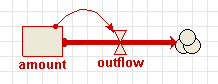
The model

Model mathOptimize
			Enumerated types: []
		 
		Variable   x
			x = 		Variable parameter 
			Minimum = 0, Maximum = 10
		 
		Variable   y
			y = 		x^3* exp(-3.0*x)

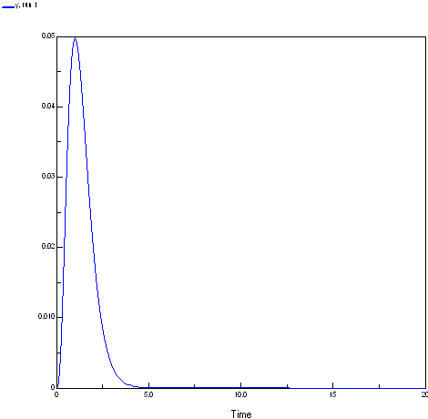
The response function of the model is shown below. To produce the plot the x values were set to the current simulation time.

The script

This script optimises the model output at the end of a run varying one input parameter. The script depends on math::optimize and uses the Plotchart package for a simple plot of the function output for a regular series of inputs the easiest way to get these package is probably to install ActiveTcl.

http://www.activestate.com/products/activetcl/

# This works to optimise for the last value of models runs.
	# The model is run for a set period (SetExecuteFor) and a parameter is set 
	# to a given value at the start of the run.
	# 
	
	# this script depends on math::optimize and uses the Plotchart for a
	# simple plot of the function output for a regular series of inputs
	# the easiest way to get these package is probably to install ActiveTcl
	# http://www.activestate.com/products/activetcl/
	
	
	# Where the extra libraries live MODIFY FOR YOUR CASE
	lappend auto_path {c:/program files/tcl/lib}; # eg ActiveTcl directories

	package require math::optimize
	package require Plotchart
	
	# Simulistics provided package
	package require SimileAutoObj; # not actually needed in Windows using SimileScript.exe
	
	
	# Create a Tcl object/command (modelWin) with which to control that instance of Simile
	similescript::ModelWindow modelWin
	
	# Tell Simile not to use the single window Model Run Environment
	# We are not going to use any helper anyway here.
	# We then load the model and build it using C++
	modelWin UseMRE false
	# MODIFY FOR YOUR CASE      MUST BE FORWARD SLASHES EVEN UNDER WINDOWS!
	modelWin Open "H:/mathOptimize.sml"
	modelWin Run
	
	
	# Create a runControl command/object with which to control
	# (as you might expect) the run control.
	similescript::RunControl runControl
	
	runControl SetExecuteFor 1
	runControl SetTimeStep 1 1
	
	# Create proc to run model and return value of variable to optimize
	proc func {x} {
	    runControl SetValue /x $x
	    runControl Reset
	    runControl Start
	    # multiply the value by -1 as we want the maximum value using a minimising optimiser
	    set y [runControl GetValue /y]
	    return [expr -1*$y]
	}
	
	package require Plotchart
	
	toplevel .t
	canvas .t.c -background white -width 400 -height 200
	pack   .t.c -fill both
	
	#
	# Create the plot with its x- and y-axes
	#
	set s [::Plotchart::createXYPlot .t.c {0.0 20.0 2.0} {0.0 0.05 0.01}]
	$s title "Shape of function we are evaluating"
	
	# evalute the model output for a range of input values ()
	# by plotting the output value for a series of input values
	# # multiply the value by -1 to get the original sign
	puts "Function shape"
	for {set i 0} {$i<=20} {incr i } {
	    set x [expr {$i/2.0}]
	    set y [expr {-1*[func $x]}]
	    puts "$x $y"
	    $s plot series1 $x $y
	}
	
	#puts "Maximum at(negative y value): [::math::optimize::min_bound_1d func 0.0 10.0]"
	set results [::math::optimize::min_bound_1d func 0.0 10.0 -trace on]
	set x [lindex $results 0]
	set y [expr {-1*[lindex $results 1]}]
	puts #####################################################
	puts {::math::optimize::min_bound_1d func 0.0 10.0}
	puts "Maximum at: $x = $y"
	puts #####################################################
	puts ""
	
	set results [::math::optimize::min_unbound_1d func 0.2 0.7 -trace on]
	set x [lindex $results 0]
	set y [expr {-1*[lindex $results 1]}]
	puts {::math::optimize::min_unbound_1d func 0.2 0.7}
	puts #####################################################
	puts "Maximum at: $x = $y"
	puts #####################################################

Results

You can see its search for the minimum if the trace is on:

(Run) 159 % ::math::optimize::min_bound_1d func 0.0 10.0 -trace on
	f(3.8196601125) = -0.000588169133818 (initialisation)
	f(6.1803398875)=-2.09302565156e-006 (golden section)
	f(2.360679775)=-0.0110514849929 (golden section)
	f(1.4589803375)=-0.039018178181 (golden section)
	f(0.901699437495)=-0.0490203182137 (golden section)
	f(0.178385003365)=-0.0033239934159 (parabolic interpolation)
	f(0.625417908211)=-0.0374683267348 (golden section)
	f(1.05516631149)=-0.0495683007526 (parabolic interpolation)
	f(1.01193600577)=-0.0497765137855 (parabolic interpolation)
	f(1.00189882668)=-0.0497867994449 (parabolic interpolation)
	f(0.99971913441)=-0.0497870624755 (parabolic interpolation)
	f(0.999993651474)=-0.0497870683649 (parabolic interpolation)
	f(1.00000018344)=-0.0497870683679 (parabolic interpolation)
	f(0.999999991611)=-0.0497870683679 (parabolic interpolation)
	f(0.999999891511)=-0.0497870683679 (parabolic interpolation)
	f(0.999997508029)=-0.0497870683674 (golden section)
	f(0.999998981102)=-0.0497870683678 (golden section)
	f(0.999999543765)=-0.0497870683678 (golden section)
	f(0.999999758684)=-0.0497870683679 (golden section)
	f(0.999999658584)=-0.0497870683679 (golden section)
	0.999999658584 -0.0497870683679

Maximum at: 0.999999658584 = 0.0497870683679

Files

• Simile model MathOptimize.sml
• SimileScript MathOptimize.tcl

You don't need to have an in-depth knowledge of Tcl to automate running Simile models using SimileScript. Generally if you have some scripting or programming experience you will be able to adapt one of the examples scripts (in the "examples" subfolder of your Simile directory). However, to understand fully what's going on in the examples you will need some more information on Tcl.

Furthermore, Tcl is a powerful language with many extensions. Powerful enough to be used for application programs, indeed the Simile user interface is written in Tcl (with Tk the graphical toolkit). If you wish, your SimileScripts may be far more powerful and complicated than the simple examples included with the Simle installation.

• Tcl Tutorial (NB the SimileScript program  (with Simile for Windows), or Wish in the Simile installation bin folder for other operating systems, should be used instead of tclsh as directed in the tutorial.)