Individual-based modelling of a population of trees
Introduction
The main aim of this tutorial is to introduce you to individual-based modelling.
System Dynamics (or “compartment-flow”) modelling generally does not represent individuals in a population. Instead, all the individuals are lumped together and represented by a single value: the number of individuals in a population, the total weight of all the individuals, or the total amount of some substance they contain (water, carbon or nitrogen, for example).
However, there are many situations when it is important to represent each individual in the population separately. For example, the behaviour of the whole population may be partly a product of interactions between individuals, or between individuals and their environment.
In this tutorial, we will look at how to model a population in terms of a set of individuals — in this case, trees. We will not consider how to handle interactions. Another tutorial, involving the modelling of the interaction between trees and crops, will be available shortly. However, we will see how to specify a set of individuals, how to give them individual behaviour (growth), and how to represent the creation of new trees and the death of existing ones.
Stage 1: Modelling the growth of a single tree
| Step 1 |
Add a compartment to the desktop, and rename it size.
|
| Step 2 |
Draw a flow into the size compartment, and rename it growth.
|
| Step 3 |
Add a variable to the desktop, above the growth flow, and rename it gr.
|
| Step 4 |
Draw an influence arrow from both the size compartment and the gr to the growth flow.
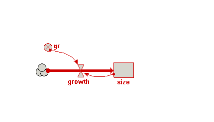
Your model diagram should now look like this:
|
| Step 5 |
Enter the following expression for the growth flow: gr*(1-size/25)
In this expression, the value 25 is the maximum size the tree will reach. It’s growth rate will fall from the maximum given by gr at the start of the simulation. This form of mathematical expression is a convenient way of achieving this desired behaviour of rapid initial growth reducing as the final maximum size is reached. |
| Step 6 |
Set the initial value for the size compartment to 3.
|
| Step 7 |
Set the value for the variable gr to 0.2.
|
| Step 8 |
Prepare the model for running.
|
| Step 9 |
Set up a plotter display helper for the size compartment
|
| Step 10 |
Run the model
|
Stage 2: Extending the model to represent a population of trees
| Step 1 |
Draw a submodel box to completely enclose your model diagram.
|
| Step 2 |
Rename the submodel tree.
This submodel will represent a population of trees. However, rather than calling it “trees”, it is conventional to name the class of objects after one individual, so here we call it “tree”. |
| Step 3 |
Open up the submodel Properties dialogue window.
|
| Step 4 |
Click the radio button labelled “Using population symbols”.
|
| Step 5 |
Choose a nice background colour for the submodel.
|
| Step 6 |
Close the submodel properties dialogue window.
Your model diagram should now look like this:
Note that the submodel boundary now has an extra line on the top-and-left, and on the bottom-and-right. This is a visual signal that Simile now represents this as a “population submodel”. |
| Step 7 |
Change the expression for gr from its current value (0.2) to rand_const(0.1,0.3).
Since we will now be simulating the growth of several trees, we are giving each one a different growth rate, randomly selected between 0.1 and 0.3. This could reflect, for example, differences in the soil conditions where each tree grows, or genetic differences between trees. |
| Step 8 |
Add a
 creation symbol to the model diagram, and give it a value of 5. creation symbol to the model diagram, and give it a value of 5.This is used to specify the initial number of trees (i.e the number at time zero). If we didn’t put this into our model, then our population would start off empty, i.e. with no trees. |
| Step 9 |
Add an
 immigration symbol to the model diagram, and give it a value of 2. immigration symbol to the model diagram, and give it a value of 2.We are stating that two new trees are created every year. |
| Step 10 |
Add a
 loss symbol to the model diagram. loss symbol to the model diagram. |
| Step 11 |
Rename the loss symbol death.
|
| Step 12 |
Draw an influence arrow from the compartment size to this symbol.
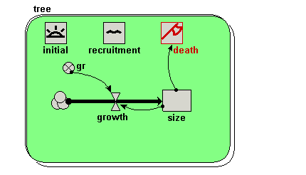
Your model diagram should now look like this:
|
| Step 13 |
Enter the expression size>17 for the symbol labelled death.
This states that a tree will “die” (be eliminated from the model) when its size exceeds 17. |
| Step 14 |
Rebuild the model, and run it again.
You should see multiple lines on the graph. Each line represents the growth of a single tree. Note that each line has a different slope, since each tree has a randomly different growth rate (as determined by the variable gr). Note also that each year two new trees are created, and that trees disappear when their size value exceeds 17. |
Stage 3: Calculating aggregate information
| Step 1 |
Add a variable outside the tree submodel, and rename it total.
|
| Step 2 |
Draw an influence arrow from the compartment size inside the tree submodel to the variable total.
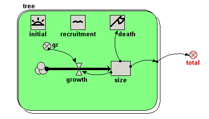
Your model diagram should now look like this:
Notice how the influence arrow crosses the submodel boundary. |
| Step 3 |
Enter the expression sum({size}) for the variable total.
Be very careful to get the brackets right. The outer (round) brackets enclose the argument for the built-in function sum( ), which can find the total value of an array of a list. In this case, we want the sum( ) function to find the total value of a list of size values, one for each tree. It’s a “list” rather than an “array” of values, because the number of trees (and hence the number of values to be summed) is not fixed, but changes over time. Simile uses braces {....} to denote a list, and square brackets [....] to denote an array. |
| Step 4 |
Re-build the model.
|
| Step 5 |
Call up a plotter display for the variable total.
|
| Step 6 |
Run the model again
In additional to the plot for the growth of individual trees, you should see a graph with a single line for the total size of all the trees, rising smoothly up, then bouncing around an asymptotic value. Why does it show this behaviour? First, trees are growing and more are being added, with none dying. Later, the growth of existing trees and the addition of new (small) ones is balanced by the sporadic death of big trees. The top of the curve is not smooth because the time it takes for a tree to die depends on its growth rate, which is randomly determined. |
Stage 4: Visualising the trees in space
| Step 1 |
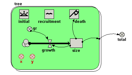
Add two variables inside the tree submodel, and rename them x and y.
|
| Step 2 |
Enter the following expression for the variable x: rand_const(0,50)
We imagine a 1 hectare plot, with the trees on the left-hand side: i.e. their x-coordinate is between 0 and 50 m. The actual x-coordinate for each tree is randomly determined. |
| Step 3 |
Enter the following expression for the variable y: rand_const(0,100).
The trees can be anywhere between the front and the back of the 1 hectare plot. Hence, the y-coordinate for each tree is randomly determined between 0 and 100 m. |
| Step 4 |
Re-build the model.
|
| Step 5 |
Call up the lollipop display. When it prompts you for the three variables required to set up the display, click on the variable x, the variable y, and the variable size respectively, in that order.
You should see a gridded area, with five lollipops on it, representing the five trees created at initialisation time. |
| Step 6 |
Run the model again.
Now, you can the trees growing, new trees being created, and trees dying off when they reach the threshold height. Note that we have not changed the mathematical nature of the model. All we have done is to change the way we visualise its behaviour — but this has a dramatic effect on our appreciation of what’s going on. |


The variable gr represents the maximum rate of growth of the tree.