The SimileScript language is object based. There are commands to create model window objects, run control objects and table display objects. Once an object is created, methods (or commands) of those objects can be used. (To those who know TclTk, the commands follow the same rules as the Tk graphical user interface widget commands.)
Model window
Create model window object
similescript::ModelWindow objectName
For example:
similescript::ModelWindow modelWin
objectName commands (or methods in object based terminology) can now be used.
Model window object commands
Most of these commands correspond to Simile model window menu commands.
objectName Open modelFile
Load (open) an existing model file from disk. It takes one argument, modelFile, that is the file name of the model to be loaded. Only one model may be loaded at any time. To remove the current model use: objectName New (see below).
Removes any existing model loaded (opened). This command corresponds to the Simile model window <strong>File</strong> -> <strong>New</strong> command. Removing the current model allows another model to be loaded.
Opens a file open dialog box, allowing the script user to choose the model to load (open)
at script run-time.
objectName LoadParams filepath ?smPath?
In order to run a model with file parameters use the command above before building the model. The filepath refers to a parameter metafile (.spf) which contains values or references to other files. smPath (submodel path) can be omitted if the parameter variables specified in the file are relative to the top level of the model.
bool must be either “true” or “false” (or other versions of Boolean values accepted by Tcl). If “true” the single-window Model Run Environment is used. Otherwise, seperate windows will be produced for each helper (display). This command is only of use if the helpers are made visible.
(New in v5.5) Returns all the enumerated type definitions in the top level of the model, in the form of a nested list. Each sublist has the type name for its first element, and the type members for its remaining elements.
objectName GetEnumTypeMembers typeName
(New in v5.5) Returns a list of the members of the enumerated type given by typeName, if it exists in the top level of the model.
objectName ChangeEnumType typeName member...
(New in v5.5) Changes the membership of the enumerated type given by typeName, if it exists in the top level of the model. The new members are the second and any subsequent arguments passed to this function. The model must be rerun before the new definition takes effect.
Makes a loaded model runnable.
Makes a loaded model runable using Tcl as the model execution environment. Tcl is slower than the usual compiled C++ executable but has more error checking. However, error checking (dubugging) is usually done from the graphical Simile user interface.
Makes the model window visible.
Hides the model window (default).
Removes the model window.
Run control
Create run control object
similescript::RunControl objectName
For example:
similescript::RunControl runControl
objectName commands (or methods in object based terminology) can now be used.
Run control object commands
Most of these commands correspond to edit fields and buttons on the regular Simile run control dialog box.
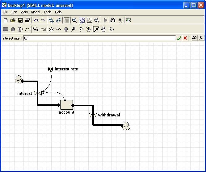
Path - Some of the methods (commands) below take a parameter path. Model component paths end with the name of the component (e.g. compartment, variable or
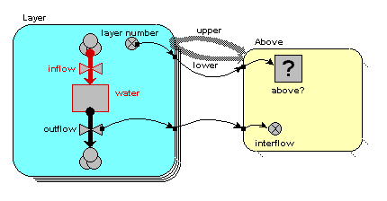
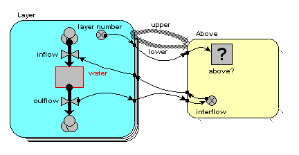
submodel preceeded by a string of all the submodels the component is contained by. The submodels are seperated by a slash “/”. The toplevel model (sometimes called the “desktop”) is refered to as “/”. Since all components are contained by the toplevel model all paths start with a leading /, e.g. “/Number of Trees” is the variable “Number of Trees” in the top level model. “/Tree/Saplings” is the variable “Saplings” in the submodel “Tree” which is contained directly by the toplevel model.
Start running the simulation. The simulation will run for the time set by, objectName SetExecuteFor, or the default execution time stored in the model file. Generally, your script will be clearer if you always use objectName SetExecuteFor. Returns a string containing the elapsed real-time to run the simulation (not CPU time), e.g.
1.27 sec
Resets the simulation to time zero.
objectName SetExecuteFor time
Set the simulation time for which the simulation will run when objectName Start is called.
objectName SetIntegrationMethod method
Set the integration method. method may be either, “Runge-Kutta” or “Euler”
objectName SetIntegrationMethodEuler
Sets the integration method to Euler
objectName SetIntegrationMethodRungeKutta
Sets the integration method to 4th-order Runge-Kutta.
objectName GetStepAdaptLimit
New to Simile v5.8: Returns the current maximum proportional error used for adaptive stepsize variation. If adaptive step size variation is not in use, a value of zero is returned.
Sets the integration method to 4th-order Runge-Kutta.
objectName SetStepAdaptLimit errorLimit
New to Simile v5.8: Sets the current maximum proportional error used for adaptive stepsize variation. If an argument of zero is supplied, adaptive stepsize variation is turned off, otherwise it is turned on.
objectName SetTimeStep index timestep
Different submodels in a model can be specified as operating on different time steps (in the submodel properties dialogue). Use this command to set timesteps.
objectName SetTimeUnits units
This setting is for use with physical units, to specify the particular time unit, rather than using abstract time units. If you have not specified consistent physical units for all flows, you should not change this setting from the default “unit”. If you have specified consistent physical units, you should choose the unit you wish to use to specify how long to execute the model for. Valid values are; unit, second, minute, hour, day, week, month, year and Ma.
objectName SetDisplayInterval timeStep
Set the simulation time interval at which displays (helpers) are updated.
objectName SeedRandoms integer
New to Simile v6.4: Initializes the state of the random number generator. This can be used to ensure that a model run produces exactly the same results each time, even if it contains random functions. The argument is used to build a state for the generator, so using the same argument will ensure the same subsequent sequence of randoms.
objectName GetCurrentTime
Returns the current simulation time.
objectName GetDisplayInterval
Returns the simulation time interval at which displays (helpers) are updated.
Returns the simulation time for which the simulation will run when objectName Start is called.
objectName GetIntegrationMethod
Returns the current integration method.
objectName GetNumberOfTimeSteps
Returns the number of different time steps used in the model.
A synonym for GetNumberOfTimeSteps.
objectName GetTimeStep index
Return the time interval for the given timestep index.
Returns the current time units.
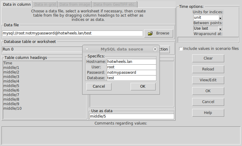
Return the value of a model variable given by the variable path path
objectName RequestValues ?path ...?
New to Simile v5.6: Requests that on each display update, a call be made to a procedure defined in the script, passing the values of the variables specified in the path arguments. If there are no arguments, there will be no callbacks. The procedure ReceiveValues is called, with the objectName making the request as the first argument, the model time as the second argument, and the values of the requested variables as the subsequent arguments.
objectName MergeParams filepath ?smPath?
This command is analogous to the model window object's LoadParams command. Once a model is made runnable (by calling simileScript::ModelWindow Run) then in order to run a model with different file parameters, use the command above before resetting the model. The filepath refers to a parameter metafile (.spf) which contains values or references to other files. smPath (submodel path) can be omitted if the parameter variables in the file are relative to the top level of the model.
objectName SetValue path value
Set the value of a model variable given by the variable path path. This only makes sense for variable parameters. Constant parameters are set by scenario file and other variables are calculated each time step.
objectName GetMaxValue path
Returns the maximum value acceptable for the variable parameter given by path. (Values are returned for variables other than variable parameters but the values are not used.)
objectName GetMinValue path
Returns the minimum value acceptable for the variable parameter given by path. (Values are returned for variables other than variable parameters but the values are not used.)
objectName GetModelClass path
Returns the class of the model component given by path. The class will be one of: SUBMODEL, VARIABLE, COMPARTMENT, FLOW, CONDITION, CREATION, REPRODUCTION, IMMIGRATION, LOSS or ALARM.
objectName GetModelDims path
Returns the dimensions of a model component given by path. Components of a variable instance submodel (population submodel)
objectName GetModelEval path
Returns evaluation method of a model component given by path. The evaluation method will be one of EXOGENOUS, DERIVED, TABLE, INPUT,
SPLIT or GHOST.
objectName GetModelType path
Returns the type of a model component given by path. The type will be one of: VALUELESS, REAL, INTEGER, FLAG or EXTERNAL. FLAGs are Boolean types.
Returns a Tcl list of all model components (e.g. submodels as well as variables). E.g. {/Number of Trees} /r /Tree/Saplings /Tree {/Tree/Tree Size} {/Tree/Growth Rate}
{/Tree/Maximum Growth Rate} {/Tree/Chance of Death} {/Tree/X Position} {/Tree/Y Position} /Tree/ID
Note that paths with spaces will be returned wrapped by { }.
Make the run control dialogue box visible.
Hide the run control dialogue box.
Table helper object
Create table helper object
Version 5 and up
similescript::TableHelper objectName run_control_object window_title
Version 4
similescript::TableHelper objectName model_window_object window_title
For example:
Version 5 and up
similescript::TableHelper tableHelper runControl "table1"
Version 4
similescript::TableHelper tableHelper modelWin "table1"
Table helper object commands
objectName AddVariable path
Adds the variable given by path to the list of variables to be written to the table.
objectName RemoveVariable path
Removes the variable given by path from the list of variables to be written to the table.
Causes the table to be updated. Use in conjunction with objectName SetUpdateAtDisplayInterval value.
objectName SetUpdateAtDisplayInterval value
If value is “true” the table updates its display every display interval (even if the table is hidden and so not visible on the screen). This takes a significant time and so the simulation will run faster if value is “false”. Use objectName Update to update the table at the end of the simulation.
objectName GetUpdateAtDisplayInterval
Return “true” or 1 if the table is set to update its display every time interval or “false” or 0 if the table does not update its display. If “false” use objectName Update before saving the contents to file or viewing the table.
objectName SetShowingRowsForTimes value
If value is “true” the table keeps a set of values for each time at which the contents are updated. This can create a large table which takes a significant time to update. If value is “false”, the table will contain only the set of values from when it was last updated. Use objectName AppendToFile to write these to file so they are gathered throughout the simulation.
objectName GetShowingRowsForTimes
Return “true” or 1 if the table is set to keep values for each time at which the contents are updated, or “false” or 0 if the table is set to show only current values. If “false” use objectName AppendToFile to save the contents to file without overwriting previous values.
Clear the table.
objectName SaveToFile filename
Save the table contents to a comma separated values (CSV) file named filename. Remember to call objectName Update if objectName SetUpdateAtDisplayInterval was set to “false”.
objectName AppendToFile filename section_id
Append the table contents, preceeded by a line containing section_id, to a comma separated values (CSV) file named filename. The file will be created if it does not already exist. Remember to call objectName Update if objectName SetUpdateAtDisplayInterval was set to “false”.
Make the table display visible.
Hide the table display.
 You start Simile by double-clicking on the desktop icon created during installation, or by clicking on the Simile icon in the Start Menu.
 compartment symbol in the toolbar.
 flow symbol in the toolbar.
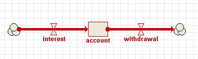
 variable symbol in the toolbar.
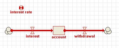
 influence arrow button in the toolbar.
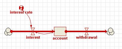
 pointer button in the toolbar.
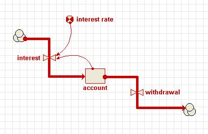
 pointer button in the toolbar.
 green tick mark or press the Return key.


 Compartment

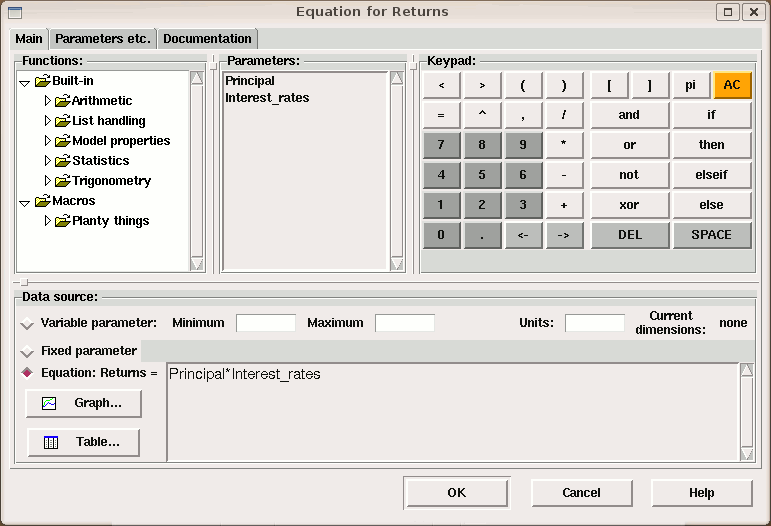
 Parameter (a coefficient in an equation): e.g. the reproductive rate per individual animal. Could also be a site constant: e.g. elevation above sea level. Its value will remain constant throughout a simulation run.
 Input lever: a
  Calculation order


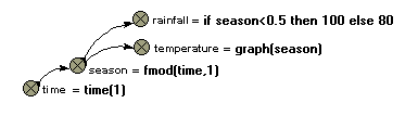
 Limit event : This represents an event that occurs when a model value reaches some pre-set limit. It requires an equation and a minimum and/or maximum value to be entered. The event occurs when the value of the equation reaches the minimum or maximum, and the event should cause the value to go no further in that direction. The event is boolean (i.e., has no magnitude) if only one limit is present. If both are present its magnitude is -1 at the lower limit and 1 at the upper limit. Hence its equation does not affect its magnitude, only its time of occurrence.
 Time series: This gets its values from outside the model like a
  'zap' button.
 pointer). This window can be kept on the screen while you scroll the main model diagram to some other part of the model. Also, you can change the
  Single role arrow
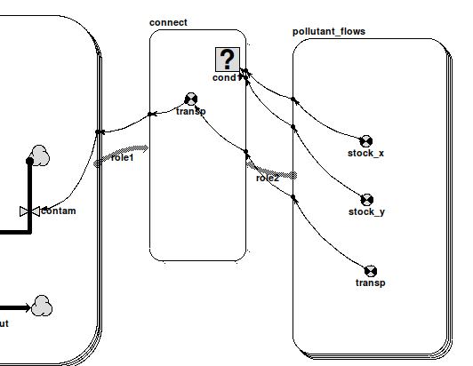
 condition symbol
 Two role arrows from different submodels
 condition symbol
 Two role arrows from the same submodel
 condition symbol
 Iteration


 variable
 compartment
 image element also behave as node-type elements, though no node is associated with them. The following procedure is used to add node-type elements.
 submodel symbol in the tool bar.
 Duplicating elements
 pointer tool on the tool bar.
 copy and
  paste commands.
 Moving model diagram elements around
 pointer tool if not already selected.
 Moving flow or squirt valve symbols
 Moving influence arrows
 move tool, when applied to submodels.
 Deleting elements from the model diagram
 pointer tool of not already using it.
 select tool on the toolbar.
 Compartments
 Flows
Flows Simple submodels
 Role arrow
 Creating ghost elements
 "Find" calls up a dialogue box into which you enter the text, and specify which text elements to search
 "Find Next" searches for successive occurrences of variables satisfying your search criterion

 select tool to double-click within a blank area, within the submodel if you have added one, or if not, anywhere on the desktop. This invokes the
  pointer mode, holding the pointer over any model component will cause a popup window to appear including that component's equation, value(s) (while the model is running) and description and comments. These can be suppressed by unchecking any or all of these options. If none is selected, the popups are suppressed completely.

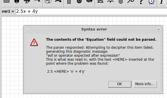
 button, or hit return, to set the equation.
 button if you make a mistake. It restores the previous entry.
 button.
 button. The top level of this cascade also contains an entry labelled "Enum. type constants", for adding the names and members of any


 pull-down menu button on the
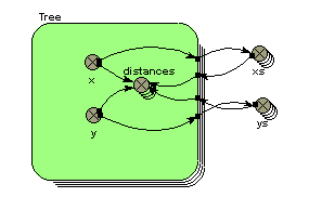


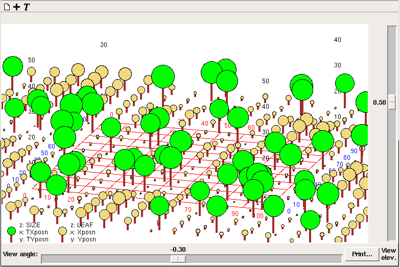
 Array-valued components
 select mode, or by using the "Properties" command of the


 creation,
  reproduction,
  immigration and
  extermination.
 Pointer tool, then double-clicking anywhere in the blank area of the submodel (not on its border, and not on any existing elements). Note that the "Generated set" radio button has been selected by default. This term denotes that the submodel is to be fixed-membership. Enter a value into the "Dimensions" box corresponding to the number of instances you want. Click on the "OK" button.
 Pointer tool, then double-clicking anywhere in the blank area of the submodel (not on its border, and not on any existing elements). Click on the "Population" radio button. Do not enter a value into the "Dimensions" box. You can use the Creation symbol to specify the initial number of individuals in the population. Click on the "OK" button.


 the
the  the
the  the
the  save button on the tool bar.
 open button on the tool bar.
 new configuration can be selected, to remove all the currently displayed helpers.


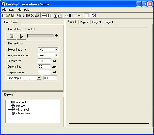
 play button will begin execution at the current time for a number of time steps set using "Execute for".
 stop button will stop the simulation (if one is running) and set the current time to zero.
 pause button will pause the simulation at the current time.
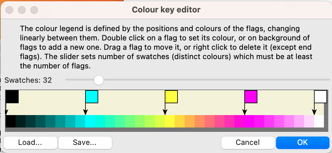
 Black
Black Purple
 Yellow
 Green
Green Blue
Blue Red
Red Grey
Grey White
White Using the
  Using the
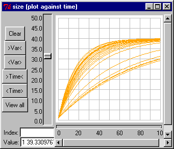
 Saving table data


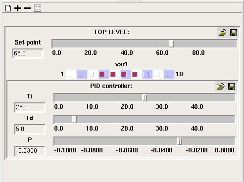
 add button to add a slider for a model component if it is a fixed or variable parameter. The - button allows you to remove the slider for a particular model component. The
  "add all variables" button will add sliders for all model components marked as variable parameters, as it is for these that sliders are most usually required. The Clear button will remove all sliders. Sliders are grouped by submodel, if their variables are in different submodels.
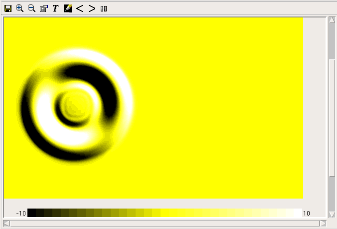


 Inspect model variable
 ) which will refresh the displayed data with the current values from the model.
 ) and select a file name. Then start the model executing. The values displayed in the snapshot window will not change, but after each display interval the current values will be appended to the file. In this case the indices will be listed in rows at the top of the file, outermost first, with the actual data items appearing below them, one row for each time point. The times themselves will appear in the leftmost column. To stop logging, hit the log button again.
 Fixed parameter
 Variable parameter
 paper roll behind its usual appearance.
 properties button in the toolbar of the model run environment.
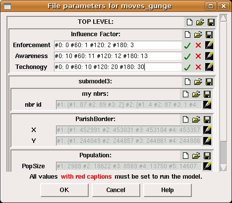


 ‘Default case’ heading, indicating that these values correspond to the ‘real world’. There is also an
  ‘Experimental conditions’ heading, with an empty tree. This tree can be built up by adding experimental cases.
 variable parameter, in which case the data for it will be an alternating list of time points and values to apply at those times. Once you have selected a parameter, an entry field for it will appear under the Experimental conditions header, as part of a new tree.
 List for parameter
 Multi-factor case
 Set of permutations


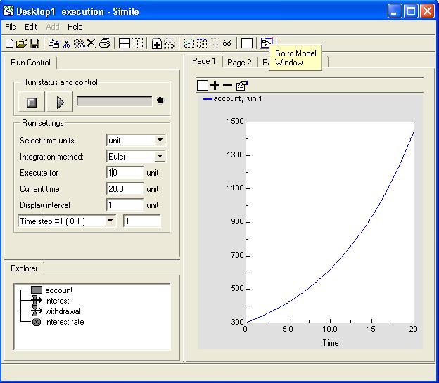
 "Go to model window" and
  "Go to run control" toolbar buttons to move back and forth between the pair.