Working with submodels
Working with submodels
Simile enables you to wrap any part of your model diagram up in a round-cornered box, called a submodel. The submodel concept can be used to address a wide range of modelling needs, including plug-and-play modularity, disaggregation, spatial modelling and individual-based modelling. If you are new to Simile, you are strongly encouraged to read the introduction to the submodel element, so that you are aware of the various uses of submodels in your modelling.
Defining properties
A submodel's properties are set using a dialogue box invoked by double-clicking anywhere within the submodel in  select mode, or by using the "Properties" command of the context menu for that submodel.
Operations on submodels
The editing operations in the context menu apply to the components in the submodel for which it was invoked. Also, the following tools are used to perform operations on submodels:
|
|
|
|
|
|
|
|
|


Advanced use of submodels
- Plug-and-play modularity uses submodels to substitute one alternative section of a model for another, or to include a model developed for another purpose or at a different time within a second model.
- Multiple-instance submodels allow a single system of components in a model to stand for many similar structures in the domain being modelled
- Conditional submodels use Boolean logic to determine the existence or otherwise of parts of the model.
- Iterative submodels contain components that are evaluated repeatedly until a finishing condition is met.
- A submodel may be given a different time step index than its parent, allowing processes in the submodel to be simulated with a shorter or longer time step than those in the parent model.
- Satellite submodels are used to extract a subset of values from a population submodel according to a given condition.
- Association submodels represent the properties of an association between two other submodels.
- Externally-supplied procedures, with array arguments and results and their own internal state, can be embodied by submodels.
- A submodel can be set up to communicate with another application.
- A spatially explicit model can be connected with a simple network model representing transport links.
In: Contents
Working with submodels : Context menu
The context menu (also known as the edit menu) can be invoked for the desktop, or for the contents of a submodel. The actions in the context menu apply only to the submodel for which it was invoked. To invoke the context menu for a submodel, either:
- Right-click in the background of the submodel while in pointer mode, or
- Click o the "Edit" item in the menu bar of a window that has been opened to display the contents of that submodel.
The context menu contains the following entries:
- Create new (only if invoked by right clicking): Creates a node-type component or starts a flow or submodelat the point selected
- Undo/Redo: only works for top level, and applies to the whole model
- Copy diagram: puts a copy of the model's graphics onto your desktop's clipboard, for pasting into other graphical applications
- Cut/copy/paste/delete: move the selected part of the diagram to or from Simile's own clipboard
- Reroute links, align to grid: tidy up the selected part of the diagram
- Select/unselect all, invert selection: Manipulate the selection to set which components other operations will be applied to
- Find, find next: search the submodel's contents for captions, equations or comments containing given text
- Properties: open the submodel properties dialogue for this submodel
- Preferences: applies to the whole of Simile
In: Contents >> Working with submodels
Working with submodels : Submodel properties dialogue
Submodel properties dialogue

The submodel properties window enables you to set the properties of a particular submodel. To invoke the dialogue box, either:
- double-click in any blank area of the submodel, or
- select the "Properties..." item in the context menu for the submodel.
The properties dialogue has two tabs, "Basic" for those most commonly used, and "Advanced" for those that are needed less often.
Basic properties
Control of number of instances
The most important property of a submodel is that it can exist in a number of different instances. Each instance follows the same logic in its calculations, but can differ in the values of its attributes. There are three mechanisms for controlling the number of instances of each submodel.
- Using specified dimensions (default)
This radio button enables you to specify that the submodel has fixed dimensions. By default, each new submodel exists only in a single instance. The dimensions can be set to be any vector or higher-order array. For example, entering 10 in the edit box, creates a vector of 10 instances of the submodel. Entering "10,10" in the edit box, creates an two-dimensional array of 100 instances of the submodel.
- Using number of data records in file
This radio button allows the number of instances of a submodel to be controlled by the number of data records in the file. The submodel must contain one or more fixed parameters, (i.e. a variable whose values are read in from a data file). The values for the fixed parameters are set in the normal way, and the number of records determines the number of instances created.
- Using population symbols
This radio button enables you to specify that the submodel is a population submodel. In this case, control of the number of instances is performed using the population symbols:
 creation,
  reproduction,
  immigration and
  extermination.
Instead of the radio buttons, Simile v6.1 includes a pulldown menu of six submodel types. When a selection is made, a message explaining the type is shown, together with entry fields for additional information required for that type. Simple (dimensionless) submodels are now separate from those with array dimensions, and there are two predefined special-purpose types: rectangular and hexagonal grid.
Background shade and/or image
These three buttons are used to specify the nature of the background colour for the submodel. The "Clear background" button specifies that the submodel is actually transparent: it will take on the colour of the enclosing submodel (or the main desktop window). (i.e. it should be read as "the background is clear", rather than the instruction "Clear the background").
The "Background shade" button calls up a standard colour selection dialogue window. Use this to select the colour of the submodel's background. This is highly recommended: having coloured submodels greatly enhances the effectiveness of the model diagram in communicating the structure of the model to other people.
The "Image…" button calls up a standard file selection dialogue window. Use this to select an image file (in either gif or jpeg formats) for the background of the submodel. There are three modes for image display:
- Tiled: If the submodel is larger than the image, the image will be repeated (tiled) across the area of the submodel; if the submodel is smaller than the image, the bottom and right of the image will be cropped to fit.
- Centred: The image will be displayed at the centre of the submodel. If the image is larger than the submodel box, only the centre of the image will be displayed. Note that a centred image will not be displayed in the background of windows showing only that submodel, because it might look confusing.
- Scaled: the image will be stretched or shrunk along each axis to fit the submodel exactly.
If a background shade as well as an image is specified, the background shade will be visible through transparent parts of the image, and also around a centred image if it is smaller than the submodel.
Appearance
- Hide contents
This suppresses the display of all model elements inside the submodel. You can do this for neatness of the diagram, so that some person looking at a complex model is spared the detail of a nested submodel. However, it is also useful if you are working with a complex model diagram, since a number of screen operations (such as deleting a model element) become quite slow with a complex model when all model elements are displayed.
- Relative scale
This changes the size of the model diagram elements in this submodel relative to those in its parent.
Description and comments
The Description and Comments boxes enable you to type in free-form comments about the submodel. Use this to document the date of creation, author, main features, etc.
Advanced properties
Calculation
The following options can be selected:
- Use units in math
This selects how physical units and dimensions are handled when checking equations in this submodel. The two mechanisms for handling units are described here. Selecting 'No' means only the first mechanism is used. 'Yes' enables both mechanisms. 'Default' uses the same setting as the submodel's parent model, or first mechanism only for the top-level model.
- Time step index
This enables you to specify on which time step the submodel is updated. In most models, there is only one time step (the "Time step #1" value in the Run Control window), which applies to all submodels. In that case, you do not need to do anything here. However, in certain circumstances, it is useful to be able to change this. See time step index for information on these cases.
The following options are alternatives to 'Build from components' which indicates that Simile should calculate the values of the submodel's components in the normal manner.
- Use own code
Allows an external procedure to read and set values in the submodel. See Using externally-supplied procedures for details.
- Conect via pipe/socket
Allows the submodel to represent a calculation carried out by another application with which Simile communicates. See Communicating with another application for details.
Enumerated types
Enumerated types are created using this dialogue box. Enumerated types are lists of names that can be chosen amongst when setting the value of a variable of that type. Please see the help page for more information on enumerated types and on how to create them.
In: Contents >> Working with submodels
Working with submodels : Opening a new window
Opening a new window for a submodel
You may want to open a new window for a submodel for one of two reasons:
- to view and edit the submodel independently of the main model
- to save the submodel to file, or load a previously-saved submodel into the current model.
You open up a new window for the submodel by selecting ![]() Pointer mode from the tool bar, then double-clicking on the submodel envelope. Note that it is fairly easy to miss, and click inside the submodel. In that case, the submodel properties dialogue will appear. If that happens, click "Cancel" and try again.
Pointer mode from the tool bar, then double-clicking on the submodel envelope. Note that it is fairly easy to miss, and click inside the submodel. In that case, the submodel properties dialogue will appear. If that happens, click "Cancel" and try again.
Note that any changes you make to the submodel in its own window are simultaneously made to the submodel in the desktop window. You can edit the model diagram using the same set of tools as are available in the desktop window. Note however, that the toolbars may not be displayed if the window is not large enough. All the tools must then be accessed through the menus.
Note also that any actions that change the scroll region of the new window, for instance growing it beyond its current scroll region, will alter the scale of the submodel relative to its parent. To understand this, consider the following terminology:
- The submodel panel is that part of the main desktop window occupied by the submodel, i.e. that is enclosed in the submodel envelope.
- The submodel window is the separate window opened up for viewing and editing the submodel.
- The submodel scroll region (also called the canvas) is the area behind the submodel window that is available for the submodel diagram.
Thus, the submodel window reveals part of the canvas. We can move around the canvas by scrolling the window with the side and bottom scroll bars. Only if the window is actually the same size as the canvas, will not need to scroll the window to see the whole canvas.
Note, now, that the submodel canvas always represents the same area as the submodel panel. Thus:
- if you increase the size of the submodel canvas, then the size of model-diagram elements in the submodel panel will decrease, relative to the other elements in the desktop window; and
- if you increase the size of the submodel panel, and use the
 zoom to fit option for the submodel window, then the size of model-diagram elements in the submodel panel will increase, relative to the other elements in the desktop window.
In all cases, however, you can also adjust the relative scale of the submodel without opening up a separate window for it, by using the relative scale slider in the submodel dialogue window.
In: Contents >> Working with submodels
Working with submodels : Saving a submodel to file
Saving a submodel
In order to save a submodel to file, open a new window for the submodel, then select the "Save" command on the "File" menu of the submodel window.
The submodel will be saved as a .sml file. In fact, this file will contain nothing to indicate that it is a submodel: Simile makes no distinction between a main (top-level) Simile model saved to file, and a submodel saved to file. If the submodel had influences coming into it from other parts of the model, then the influenced variables in the submodel will be converted to "Input Parameters", indistinguishable from input parameters in top-level models specified by the model designer. The only thing to note is that these automatically-created input parameters will appear red in the model diagram if you have not specified "Min" and "Max" values for them in the equation dialogue prior to saving the submodel.
In: Contents >> Working with submodels
Working with submodels : Importing a submodel from file
Loading a saved model as a submodel
In your current model, create an empty submodel. This should be fairly large, so that the diagram of the model you will be inserting is not all squashed up.
Select ![]() pointer mode, and double-click on the boundary of the submodel. (If you miss, you will see the submodel properties dialogue window: cancel this and try again). You will see a new model diagram window, just like the main desktop window except smaller. It will have the same menu as the main desktop window.
pointer mode, and double-click on the boundary of the submodel. (If you miss, you will see the submodel properties dialogue window: cancel this and try again). You will see a new model diagram window, just like the main desktop window except smaller. It will have the same menu as the main desktop window.
Select the "Open" command from the "File" menu, and locate and load the Simile model (.sml) file.
You will see the loaded model in both the new submodel window, and in the round-cornered submodel box in the main Desktop window. You can close the submodel window, or keep it there if you want to work on the submodel and it is too small in the main Desktop window. Note that, if you enlarge the submodel window, you will probably want to do Zoom to fit in order to get the model submodel diagram to occupy the whole of the available space.
Any model or submodel saved to file can be treated as a submodel or as a model. No real distinction is made between the two concepts. If you load a previously-saved model into a submodel window, then it will become a submodel in the current model. If, on the other hand, you load a previously-saved submodel into the desktop window (i.e. the main, top-level window), then it will become a model in its own right.
So, in order to load a previously-saved submodel as a stand-alone model, all you need to do is to start a new session of Simile (or select the "New" command from the "File" menu in the desktop window), then select the "Open" command from the "File" menu in the desktop window, and find the .sml file that contains the previously-saved submodel.
Any variables in the submodel that had previously received influences from outside the submodel automatically become "Input parameters". If they had been previously assigned min and max values, then you will get a slider for each such variable when you come to run the submodel (now a model). Any such variable that had not been assigned minimum and maximum values will appear red when you load the submodel, and you need to open up the equation dialogue for this variable and either:
- unclick the "Input parameter" check box and enter a value into its equation dialogue; or
- enter min and max values.
In: Contents >> Working with submodels
Working with submodels : Multiple-instance submodels
Multiple-instance submodels
Multiple-instance submodels are one of Simile's most valuable features, for constructing object-based models. For real-world objects, such as a tree, it is useful to be able to model several particular instances of the object, each acting in the same general way, though differing in their particular attributes.
- Fixed membership submodels have a specified number of instances
- Per-record submodels have one instance for each set of data loaded for its parameters.
- Population (variable membership) submodels offer control over the number of instances using special model elements
- Special-purpose submodels have many instances, and extra features which assist in modelling particular common phenomena, e.g., spatial grids
Working with submodels : Multiple-instance submodels : Fixed
Multiple-instance submodels: fixed membership
A fixed-membership submodel is one type of multiple-instance submodel. In this case, the number of instances is fixed throughout the simulation run.
By making a fixed-membership multiple-instance submodel, we are saying that:
- The model contains a fixed number of objects, each of which behaves according to the same rules (represented by the model elements and equations inside it).
- Each object may (and usually does) differ in one or more numeric values: the initial value for compartments, or the values of parameters.
When should I use a fixed-membership multiple-instance submodel?
Fixed-membership submodels are useful for handling many forms of disaggregation in model design. You may, for example, be interested in modelling the changing population of a country like the UK. You first model has a single compartment, representing the total population size. You then decide to represent this information on a regional basis, in order to capture differences in population parameters in different regions. You have now disaggregated your model into multiple regions. Your model diagram looks very similar: the only difference is that the part representing population dynamics is now wrapped up in a multiple-instance submodel, one instance for each region. This is a fixed membership submodel, because the number of regions is fixed.
Conversely, fixed-membership models can be used for scaling up. To take the previous context, you might have begun making a model of the population growth of just one region. You then want to scale the model up to the whole of the UK. Again, you wrap up the original model and make it into a fixed-membership, multiple-instance submodel.
Although disaggregation and scaling up are conceptually very different - in fact, opposite - activities, the appearance of both the before and after model diagrams is the same in both cases. The only difference comes in terms of the initialisation and parameterisation for the original model.
How to make a fixed-membership submodel
- Use the submodel tool to drag a submodel envelope on your model diagram. The submodel may be drawn in an open area of the model diagram, and not enclose anything. Or you can drag the submodel around existing elements on your model diagram, if you want those enclosed in the submodel.
- Open up the submodel properties dialogue by selecting the
 Pointer tool, then double-clicking anywhere in the blank area of the submodel (not on its border, and not on any existing elements). Note that the "Generated set" radio button has been selected by default. This term denotes that the submodel is to be fixed-membership. Enter a value into the "Dimensions" box corresponding to the number of instances you want. Click on the "OK" button.
- Back on the model diagram, the submodel's appearance has now changed. Its simple border has now been replaced by multiple lines on the bottom and right, indicating that there is a fixed number of multiple instances (it's meant to look like a stack of cards).
Dimensions of a fixed-membership submodel
The dimensions of a submodel are a list of one or more dimensions, separated by commas if there is more than one. Each dimension can be:
- An integer greater than 1, or
- The name of an enumerated type, or
- size(x), where x is the name of another component in the model. The dimension then has the same value as the dimensions of the named component.
If there is just one dimension, the submodel's instances form a one-dimensional array, or vector, in which each instance has a unique index which is a number starting from one (if the dimension is numerical) or a member of the enumerated type whose name is the dimension.
If there is more than one dimension, the submodel instances are arranged in an n-dimensional array, with each instance having indices corresponding to its place long each dimension.
How to make the different instances different
There are two main ways in which you can make one instance different from the others.
- You can give each instance a different initial value for one or more compartments.
- You can give each instance a different value for one or more parameters.
Conceptually, these are very different. In the first case, you are saying that the differences between the individuals are simply in terms of the state they happen to be in when you start the simulation. In the second case, you are saying that the individuals differ in some intrinsic property. You can of course mix these: individuals may differ in both their initial state and their parameterisation.
There are several methods you can use to assign different values to different instances. These techniques apply equally to compartments and parameters.
Load the values from a file
If you put a fixed parameter inside a fixed membership submodel, then when you run the model, there will be an entry in the file parameters dialogue requiring values for this parameter. The data you enter will have to include a value for each instance of the submodel.
Generate the values randomly
Enter the expression
rand_const(0,10) (replacing 0 and 10 by whatever range you want)
in the Equation box for the compartment or parameter to cause each instance to be assigned a value randomly picked from the specified range. rand_const(A,B) samples from a rectangular probability distribution over the range A...B: Simile also alows you to use values from other distributions, e.g. Normal (and it is possible to engineer these yourselves).
Note that if there is no explicit indication that they return a constant value, Simile's statistical functions return a new sample from the given distribution on each time step. If you are using a sampling function to set up a multiple instance submodel with data that conforms to a statistical pattern, it is probable that you want each instance to keep the value it was given when the model was initialized or reset. This can be arranged by wrapping the statistical function in the at_init() function, e.g., at_init(gaussian_var(50,10)).
Select elements from an array
If your submodel has a small number of instances, you can explicitly list the value for each instance in an array, and select from this array the value for each instance.
Let's say you want to model the loss of water from 5 tanks. The tanks differ in terms of the initial amount of water they hold: say 10,5,20,50 and 9 litres. You have made the water flow model into a submodel with 5 instances. You could use the following expression in the Equation box to initialise the water compartment:
element([10,5,20,50,9],index(1)) (replacing [10,…,9] by whatever you need)
This selects the value 10 for the first instance, the value 5 for the second, and so on. See the help information on the functions element and index for more information.
Alternatively, you could have a separate array variable, say "initial_water", whose only job is to hold the array of values, take an influence arrow from it to the compartment, then select a value from that array for each instance:
initial_water = [10,5,20,50,9]
water = element([initial_water],index(1))
Use conditional expressions
You can develop expressions conditional on the value of index(1) (i.e. the numeric index of each instance) in a wide variety of ways. For example, you want the first three instances to have a value of 20, and the rest 10, then you could use the expression:
if index(1)<=3 then 20 else 10
Use a sketched graph or built-in table
You could use the sketch graph or built-in table functions in the equation dialogue to specify the values of the compartment or parameter as a function of index(1). This is particularly appropriate if the instances have a natural ordering, e.g. age-classes in a population, or soil layers, when the quantity under consideration might be considered to have some ordered relationship with the instance number.
The in_preceding() function
This calculates the value of its argument in the immediately preceding instance of the submodel. For instance, a variable with the equation in_preceding(prev(0))+1 will have a value of 1 in the first instance, 2 in the second, and so on up to the total number of instances in the last instance, irrespective of the submodel's dimensions.
Variables exported from a fixed-membership multiple-instance submodel
If you take an influence from a variable (a) in a fixed-membership multiple-instance submodel to another variable (b) in the same submodel, then b sees a as a scalar variable: i.e. as having a single value. You could use an expression for b like
3*a
How can this be, when we know that a has one value for every instance of the submodel? It's because the equation is expressed as a general rule: whatever value of a a particular instance has, then its value of x is 3 times greater.
However, things change when we take an influence from a variable (a) in the submodel to one outside (c). Because c is outside the submodel, it can see all the values of a. a must now be treated as an array of values, not as a single value.
An array is denoted by enclosing the name of the variable with [...], thus a inside the submodel has become [a] outside it. Thus, when we open up the Equation dialogue window for c, the influencing variable appears as an array, and its name is enclosed in square brackets. And the expression for calculating c must do the same. Thus, legitimate expressions for c are:
3*[a] c becomes an array with as many elements as a, each multiplied by 3
sum([a]) c has a single value, equal to the sum of the elements in the array [a]
In: Contents >> Working with submodels
Working with submodels : Multiple-instance submodels : Per-record submodels
Submodels with one instance per data record
It may be that you want to run your model with many different datasets, and these datasets each have different numbers of records which are supposed to correspond to instances of a submodel. Or perhaps you have nested submodels, where the membership of the inner submodel is different in each instance of the outer submodel, with the actual memberships being determined by the numbering of data records in a file.
For these cases, Simile provides the option of setting the number of instances according to the number of data points given for the fixed parameters within the model. To use this option, open the submodel properties dialogue and select the second radio button on the "Control of number of instances" panel, captioned "Using number of data records in file". The submodel will have the same border style as a population submodel, but should not contain any of the population control symbols. It must contain at least one fixed parameter.
When running the model, you must provide data for the fixed parameter(s). For each instance containing the per-record submodel, there must be at least one data item (the submodel must have at least one member) and the indices should run from 1 consecutively to the number of instances. You can have nested per-record submodels, possibly with the memberships of both the outer and inner submodels being set by the same parameter.
In: Contents >> Working with submodels
Working with submodels : Multiple-instance submodels : population
Multiple-instance submodels: population
A population submodel is one type of multiple-instance submodel. In this case, the number of instances may vary throughout the simulation run.
By making a population submodel, we are saying that the model contains a collection of objects, and individual objects can be created and destroyed during the course of a simulation run. The objects may (and usually do) differ in their attributes, but this is not such a central idea as it is for fixed-membership submodels: we can get interesting behaviour from a population model even if all the individuals have the same initial state and the same parameterisation.
See also the 6th video in the Simile Tutorial Series.
When should I use a population submodel?
When I introduced the idea of fixed-membership multiple-instance submodels, I said that you can decide to have one in your model either by breaking something into smaller pieces (disaggregation), or by representing a larger unit as a multiple of a set of smaller units (scaling up).
Similar ideas apply to using a population submodel, but we use slightly different language. If you are interested in the behaviour of some large unit, such as the population dynamics of the deer on an estate, then you may consider it appropriate to model this in terms of all the individual deer on the estate. This is more a process of decomposition of the population into individuals rather than disaggregation. With the latter term, the small unit is like a miniature version of the larger one, with all the same attributes, whereas an individual deer is not a smaller version of a population. Conversely, you may have first modelled one deer, following its life history, then decided to make a model with lots of those rather than just one. This is more a process of multiplication rather than scaling up. (There is no standard terminology here. Don't worry too much about the terms used: the important point is to see that something different is going on with populations.)
How to make a population submodel
- Use the submodel tool to drag a submodel envelope on your model diagram. The submodel may be drawn in an open area of the model diagram, and not enclose anything. Or you can drag the submodel around existing elements on your model diagram, if you want those enclosed in the submodel.
- Open up the submodel properties dialogue by selecting the
 Pointer tool, then double-clicking anywhere in the blank area of the submodel (not on its border, and not on any existing elements). Click on the "Population" radio button. Do not enter a value into the "Dimensions" box. You can use the Creation symbol to specify the initial number of individuals in the population. Click on the "OK" button.
- Back on the model diagram, the submodel's appearance has now changed. Its simple border has now been replaced by a double line on the bottom and right, and a double line on the top and left.
How to make the different instances different
In general, you can use methods that are the same as or similar to those used for fixed-membership multiple-instance submodels, with some differences:
- Use the channel_is() function. If your population has multiple channels (creation, immigration and reproduction symbols) then an equation can apply this function to a parameter corresponding to an influence from one of the channels to get a boolean result which is true in each individual that appeared due to that channel.
- Use the parent() function. If your population contains a reproduction symbol, an equation can apply this function to a parameter corresponding to an influence from this symbol. The result is the index number of the individual that became the parent of the current individual, or 0 if the current individual appeared due to some other channel.
- The in_progenitor() function evaluates its argument as if in the population individual whose reproduction channel caused the current individual to come into existence. For instance, in_progenitor(index(1)) is equivalent to parent().
- You cannot put a file parameter (fixed or variable) in a variable-membership submodel. This is because the table created by loading the data for a file parameter has a fixed number of values, and cannot be matched to a variable number of submodel instances.
Variables exported from a population submodel
With a fixed-membership multiple-instance submodel, variables are exported as arrays, since Simile knows precisely how many elements there are, and this number remains fixed for the duration of the simulation run. However, the number of instances for a population submodel can change dynamically during the course of the simulation run. Therefore, the set of values for a variable are exported as a list rather than an array. The number of elements in a list can vary, and (unlike an array) we can attach no particular significance to "the third element" of the list (since this might refer to quite different instances at different times during the course of the simulation)
Note that although an array can be passed around from one variable to another, a list must be processed into a scalar (single-valued) quantity as soon as it is received. Since any quantity exported from a population submodel must be a list, this means that the receiving variable must derive a single value from this list: its sum, perhaps, or its largest value, using a function capable of having a list as one of its arguments.
Special model diagram elements for population submodels
Four of the model diagram elements are only used in population submodels. They are:
 initialisation, for specifying the initial number of instances;
 migration, for specifying an absolute rate of creating new instances;
 reproduction, for specifying the rate per individual for creating new instances; and
 extermination, for specifying the conditions under which an instance is removed.
See the appropriate entries for further information on how to use these elements.
In: Contents >> Working with submodels
Working with submodels : Multiple-instance submodels : Special-purpose submodels
Special-purpose submodels
Generally, a Simile submodel has no built-in semantics besides what is described above for specifying its dimensions and how the number of instances is determined. However, certain uses of submodels are so common that we have decided to create special types of submodel to better support these uses, making models using them simpler and computationally faster. So, instead of the three radio buttons, Simile v6.1 includes a pulldown menu of six submodel types. When a selection is made, a message explaining the type is shown, together with entry fields for additional information required for that type. Simple (dimensionless) submodels are now separate from those with array dimensions, and there are two predefined types:
Rectangular grid
The submodel has two dimensions and represents rectangular patches that cover a larger rectangular area. In addition to the usual features of array submodels, rectangular grid submodels can contain the following:
- The functions row_id() and column_id() can be used to get the indices of each instance's row and column in the grid (these are equivalent to index(2) and index(1) respectively)
- An influence's properties can be edited to enable the role "Include list of values from up to 8 grid squares...". When this role is enabled, the equation of the destination component can refer to the source component values in two ways: by the normal name, which just gives the value in the same submodel instance as normal, or by the name prefixed with "from_8_nbrs_", which gives a list of values from the instances representing the 8 grid squares adjoining the current one at sides or corners. There may be fewer than 8 values, e.g., if the current square is on the side or corner of the whole grid.
Hexagonal grid
The submodel has two dimensions and represents regular-hexagonal patches that cover a larger, roughly rectangular area in a honeycomb pattern. The patches have vertical sides, and odd-numbered rows are shifted half a width to the right so they tesselate with the even-numbered rows above and below. Hexagonal grid submodels can contain the following:
- The functions row_id() and column_id(), as for rectangular grids
- The functions hex_centre_x() and hex_centre_y() which give the x and y coordinates respectively of the centre of the hexagon relative to the bottom-left corner of the grid, in multiples of the length of one side of a hexagon
- The functions hex_vertices_x() and hex_vertices_y() which give arrays of six values that are the x and y coordinates of the vertices of each hexagon, in the same terms as the centres above
- An influence's properties can be edited to enable the role "Include list of values from up to 6 grid hexagons...". When this role is enabled, the equation of the destination component can refer to the source component values in two ways: by the normal name, which just gives the value in the same submodel instance as normal, or by the name prefixed with "from_6_nbrs_", which gives a list of values from the instances representing the 6 grid hexagons sharing an edge with the current one. There may be fewer than 6 values, e.g., if the current hexagon is on the side or corner of the whole grid.
More about values from neighbours
These special influence roles are intended to replace the requirement of having a separate self-association submodel representing the neighbour relationship between members of spatial grid arrays, and moving values between neighbours by taking them out to this association submodel by one role and back by the other. The lists of values they generate are variable-membership (due to different neighbour counts at sides/corners) so must be summed or applied to some other cumulative function before being assigned to the value of a local variable. However, all the usual operations can be applied to them before this. In fact the grid cell submodel itself can be made variable-membership, by adding a condition component to it just as is done for ordinary array submodels. This could be useful if we have an irregularly shaped area that we want to break down into grid cells -- in this case, set the dimensions of the grid so it covers the whole area, then add a condition that is true only for those cells that fall into the irregular area. Cells will then have fewer neighbours if they are at the edge of the selected area, and a single 'island' cell would have no neighbours, with the neighbour influence roles supplying empty lists.
Additionally, the lists have indices from special enumerated types representing the different directions in which the neighbour can lie. For the rectangular grid these are the points of the compass: nw, n, ne, etc. For the hexagonal grid these correspond to odd-numbered hours on a clock face, and so are written 1h, 3h ... 11h. These can be used like members of any other enumerated type, and to make a multi-instance submodel in which they are the indices, the dimension should be rect_nbr or hex_nbr. Now, because Simile v6.1 also introduces the ability to use the element() function to select sublists from lists, we can get other sets of neighbour data that might be useful, e.g.,
element({from_8_nbrs_size}, ["n","w","e","s"])
will produce a list of the values of 'size' in only the neighbouring rectangles that share a whole side with the current one.
element({from_6_nbrs_fire}, ["1h", "3h", "5h"])
will produce a list of the values of 'fire' in only the neighbouring hexagons further right than the current one. Note though that this could also be done by comparing the results of the hex_centre_x() function in the local and neighbouring hexagons, e.g., is 'fire' true in any neighbour hexagon to the right? use:
any({from_6_nbrs_fire} and {from_6_nbrs_xctr}>xctr)
...where xctr is another variable with equation hex_centre_x() and an influence to the current one with values from neighbours enabled.
In: Contents >> Working with submodels
Working with submodels : Plug-and-play modularity
Plug-and-play modularity using submodels
"Plug-and-play" modularity means the ability to replace one module in a model with another, without having to specify how the module's inputs and outputs link up with the rest of the model. This requires that the modules to be swapped share the same interface to the rest of the model.
In Simile, a module is a ![]() submodel. There is a mechanism for replacing one submodel with another: simply open a separate window for the submodel, and use the File: Open command to load a new submodel. However, this by itself does not automatically remake all the links between variables in the submodel and those in the rest of the model.
submodel. There is a mechanism for replacing one submodel with another: simply open a separate window for the submodel, and use the File: Open command to load a new submodel. However, this by itself does not automatically remake all the links between variables in the submodel and those in the rest of the model.
In order to have plug-and-play modularity, we need to specify the interface between a submodel and the rest of the model. This means stating which variable in the submodel is linked to which variable in the main model, and the nature (dimensions, units) of the two variables. This specification is saved in a separate interface specification file, and can be loaded when we create a new submodel, in order to re-make all the linkages.
Demonstration of plug-and-play modularity
- Step 1: Build a model with submodels
- Step 2: Save one of the submodels as a separate model
- Step 3: Save the interface specification
- Step 4: Clear the submodel
- Step 5: Load an alternative version of the submodel
- Step 6: Load the interface specification file
In: Contents >> Working with submodels
Working with submodels : Plug-and-play modularity : Step 1
Step 1: Build a model with submodels
In this simple example, we make a model of the interaction between plant
growth and soil water. We use a submodel for each component. Note that
at this stage we do not actually need to use submodels: they merely serve
to show the main functional components of this model.

In: Contents >> Working with submodels >> Plug-and-play modularity
Working with submodels : Plug-and-play modularity : Step 2
Step 2: Save the submodel as a separate Simile model
We first open up a separate window for the soil submodel by double-clicking on its boundary.

We now select the "Save as..." command from the submodel window's File menu (not the menu for the main model window).

In: Contents >> Working with submodels >> Plug-and-play modularity
Working with submodels : Plug-and-play modularity : Step 3
Step 3: Save the interface specification
We save the interface specification for the interface between the soil
water submodel and the rest of the model, using the "Save Interface"
command from the "Model" menu of the submodel window.
In: Contents >> Working with submodels >> Plug-and-play modularity
Working with submodels : Plug-and-play modularity : Step 4
Step 4: Clear the submodel
We clear the submodel, by selecting File: New from the submodel window's
menu.

In: Contents >> Working with submodels >> Plug-and-play modularity
Working with submodels : Plug-and-play modularity : Step 5
Step 5: Load an alternative version of the submodel
We now load an alternative version of the submodel.

This new submodel also has a variable called "Soil water" (though in this case it is a Simile variable, not a compartment), and a flow called "transpiration". Note also that this submodel is structurally different from the first submodel: all that matters for plug-and-playability is that the two models have the same interfacing variables: the rest of their structure is irrelevant.

At this stage, the linkages are not re-made. The Soil submodel contains an unsatisfied input parameter "Plant biomass", while the main model contains an unsatisfied input parameter called "Soil water". These undefined elements are shown in red.
In: Contents >> Working with submodels >> Plug-and-play modularity
Working with submodels : Plug-and-play modularity : Step 6
Step 6: Load the interface specification file
We select an interface specification file using the "Load interface"
command from the "Model" menu of the submodel window (again, not the main
model window).
Now, Simile automatically re-makes the linkages between the submodel and
the rest of the model.

Finally, we can close the submodel window, since it is not required any
more. We now have the new model!

In: Contents >> Working with submodels >> Plug-and-play modularity
Working with submodels : Conditional submodels
Conditional submodels
A conditional submodel is used when there are conditions under which a submodel, or an instance of a fixed-membership multiple-instance submodel, may or may not exist. By "exist" we mean that Simile evaluates the expressions in the submodel. The existence of each instance of the submodel is determined by evaluating a Boolean expression in a  condition symbol placed inside the submodel.
The conditional submodel may represent a phenomenon that only occurs at certain times, for instance bush fires. Or it may represent a phenomenon that occurs in some, but not all, of the members of a group; for instance, if an area of interested is represented by a grid, then some vegetation types, e.g., forest, may be present in only some of the grid squares, so the processes associated with them sould be represented in a conditional submodel of the grid-square model.
If the submodel has influence arrows going from inside to variables outside itself, then:
- if the submodel exists, the values emerging from the submodel are those calculated from the variables in the normal way;
- if the submodel (or instance of it) does not exist, then a value is not exported for each variable: there is no value, since the variable just doesn't exist.
This means that we cannot be sure how many values are going to be exported from a single variable inside the conditional submodel. For a simple submodel, there could be zero or one values. For a fixed-membership multiple-instance submodel, there could be 0…n values, where n is the number of instances for the submodel.
Therefore values are always exported as a list from a conditional model, since a list (as opposed to an array) is the data structure used when the number of values in the data structure can vary dynamically over time. A list must be processed as soon as it is received: it cannot be passed around as a persistent data structure. Typically, you will simply use the sum function to add the values in the list together.
A few more detailed considerations:
- The condition equation itself, and the equations of any variables in the submodel that affect the condition, must be evaluated in every case. If the condition comes out false, the values of these variables are discarded.
- The condition cannot depend on a value outside the submodel that itself depends directly on values inside, since getting this value would require the existence status of the submodel to be already known. Simile reports this as a circularity problem.
In: Contents >> Working with submodels
Working with submodels : Iterative submodels
Iterative submodels
Motivation
System-dynamics models are usually a very naturalistic way of describing a process that takes place. The actual way in which one quantity influences another in the problem domain is mirrored by one variable influencing another in the model. If a calculation must be repeated a certain number of times with each value depending on the previous one, it can be done in a multi-instance submodel using the in_preceding() function to allow each instance to refer to values from the previous one.
However, we may wish to create a model of a system in which our best understanding of how a certain quantity is evaluated involves a procedural computation in which an instruction loop is repeatedly executed until some exit condition is met. Using a multi-instance submodel is wasteful because the number of iterations needed may vary widely, and we are not interested in values from iterations before the last one. An example is the Ball-Berry model of stomatal conductance. Although in nature stomatal conductance is the result of a purely incremental process, the easiest way to evaluate it in a model of plant physiology is to include an iterative calculation with a finishing condition. If performing a calculation like this in a procedural programming language such as c++, you would use a 'while' loop. Such a calculation could be included using Simile's ability to implement a submodel's behaviour using a piece of code in c++, but this is not ideal, since:
- One shouldn't need to learn a programming language to use Simile
- It defeats the point of the model's behaviour being visually explicit
Simile therefore allows iterative processes to be represented graphically. This involves a mechanism to specify that the components inside a submodel are evaluated repeatedly until a specified end condition is met. With this system, a modeller can not only implement iterative approximations to natural processes such as the Ball-Berry model -- they can also create graphically explicit procedures for solving abstract problems, such as finding prime numbers or efficiently sorting an array.
Implementation
An iteration symbol and a property for influence arrows are included, to allow a loop to be executed multiple times within one time step. Such looping may be required, for example, when the value of a variable cannot be calculated directly from others, but is found by trying many successive values to minimise some error function.
The basic elements of an iterative loop are as follows.
The iteration symbol contains the condition that marks the successful convergence of the iteration. An influence arrow coming from the alarm symbol can be used as an argument to the function iterations( ). This function returns the number of iterations made so far. This function can be used to set the initial value (also called the guess) for the loop, i.e. when the number of iterations so far is equal to zero. If the number of iterations so far is one or more, then the result of the last calculation should be used. Since the last calculation depends on the result calculated from the guess, a circular loop of influences is present. Normally, Simile would reject this loop at build time, but the definition of the iterations() function makes it explicit that the influence from the alarm symbol refers to its value on the previous iteration, and therefore cannot be part of a circularity.
You do not have to use the iterations( ) function; if the results of previous iterations are irrelevant, as for instance in a generate-and-test algorithm, you may not need to have any influences from the alarm symbol at all. Alternatively, if each result does depend on previous ones but the actual number of iterations is irrelevant, you can use the boolean value of the alarm symbol directly to choose between starting a new iterative approximation (true) and refining the result of the previous iteration (false). In this case you would get a circularity, but setting a property of the influence arrow: "Use values made in same time step" to true, allows the loop to be processed. You also need to set this property on influences that convey the result of the last iteration step for use at the start of the following step. Influence arrows with this property set are drawn with a dashed line, and the equation that uses their value gets the one from the previous iteration rather than the current one. To set this property for an influence arrow, double-click on it to invoke the property dialogue box.
It is unlikely that any of the above description is comprehensible without an example. The included example model for Ball-Berry stomatal conductance poses a problem for conventional System Dynamics modelling tools because it depends upon the solution of the following pair of simultaneous equations.
Gs = g0 + g1 * A * H / Ca
A = Gs * AQ
Apart from the external parameters, g0, g1, H, Ca and AQ, the equation for Gs depends only on A, and the equation for A depends only on Gs. In this implementation, the loop is opened, by introducing a place-holder for Gs, called Gs_0. This variable is calculated from A. A is calculated using Gs. A guess is made for the initial value of Gs. Subsequently, Gs is set to the last calculated value of Gs_0. The influence arrow from Gs_0 to Gs is dashed, indicating that the value from the previous iteration is to be used. The alarm symbol terminates the iterative loop when Gs and Gs_0 differ by less than one part in one thousand.
Caution
Alarm submodels should always behave as if everything in the submodel is executed repeatedly until the finishing condition is reached. However, Simile always tries to do as little work as possible, so this may not actually happen. For instance if the submodel contains constants, these are not set in each loop but set just once before the loop starts.
Also, if the exit condition in the iteration symbol does not depend directly or indirectly on a certain value in the submodel, then Simile will assume that that value is not relevant to the loop calculation and it will instead be calculated only once after the loop has finished. For instance, we made a test model that carried out a merge sort by iterating until the required number of merges were done. Since we know that for an array of n elements, the number of merges needed is log2(n), we just had a condition that counted this number of iterations. However, this resulted in only one actual merge being done rather tha a series to build sorted sublists of increasing lengths. The fix was to make the exit condition depend on the output array, to force it to be merged every cycle. This could have been done by actually checking that each value was larger than the preceding one, but it is simpler just to check for some dummy never-true condition e.g. sum([out])!=sum([out]) as well as the right number of iterations having been done.
Another problem is that if you make a mistake when building an iterative submodel, you may end up with the exit condition never being met. The model will then go into an endless loop. To escape the loop, hit 'pause' on the run control, and wait for the 'model seems to have got stuck' message -- you can then exit the model and try to fix the problem.
In: Contents >> Working with submodels
Working with submodels : Time step index
Time step index
Introduction
Specifying different time step indices for different submodels is an advanced topic. It can lead to misleading results, and should be used only in accordance with the following notes.
By default, all the model state variables are updated using the same time step. When Euler integration is used to update the state variables, differential equations are, in practice, solved as if they were difference equations, with a small but finite δt. By specifying δt , the time step, to be reasonable small, the results of the difference equations are the same as the expected results of the differential equations. You can, however, take advantage of this ability to specify δt, to use different time steps for different submodels.
A common example is in the calculation of compound interest on money in a savings account. It is important when specifying that interest is to be compounded, that the period over which the compounding occurs is specified. For example, the same investment in two savings accounts, both paying compound interest at 12 per cent, will yield different amounts after one year if one account compounds monthly and the other compounds annually. In modelling these accounts, you would need to specify a different δt, the time step, for each, in order that the state variable (the amount in the account) was updated at different rates, either monthly or annually.
Another reason for having several time steps is when a model contains components that behave on different time scales. For instance a model of a grazing system might contain a lot of plants, with physiological processes that can be modeled with a time step of a day, and animals whose movements would be modeled on a time step of seconds or minutes. To model all the plants at the shorter time step would be inefficient, so the animals are handled by a separate submodel which is run with a shorter time step.
It is possible to specify up to seven time step indices. For each new time step category that you request, an extra Time step #x entry is added in the Run Control window, and that is where you specify the actual time step (e.g. 0.01) to be used for each index.
Notes
The following notes will help you use this concept:
- Note that the TIME UNIT is the same over the whole model, and that all flows are expressed per time unit. The run control also specifies how long the model should be run for, in terms of time units.
- Each submodel TIME STEP is specified in terms of a multiple of the time unit. The submodel time steps *must* be ordered from long to short, #1 must be the longest, #7 the shortest. During each time step that affects a submodel (i.e. its own and all longer ones) all the elements of the submodel are updated. Note, particularly, that since flows are expressed in time units, a compartment's value does not change each time step by the value that is entered (or calculated) for the flow, but by the same multiple of that value as the time step is of the time unit.
- To refer to the time step in the model, use the function dt().
Special cases
In addition to the seven time step indices available, there are three special cases:
- "Initialize only" denotes that the submodel should be updated only when the model is built.
- "New params only" denotes that the submodel should be updated only when the model is built or when it is reset after new values for fixed parameters have been loaded.
- "Reset only" denotes that the submodel should be updated only when the model is built or when it is reset.
In none of these cases will the submodel be updated during the simulation.
Example
For the example of compound interest given above, set the time step index for the annual submodel to #1 and for the monthly submodel to #2. In the run control, you will then need to set time step #1 = 12 and time step #2 = 1. Flows in both submodels will be expressed in the same time units, in this case, per month.
Note that this is exactly equivalent to time step #1 = 1 and time step #2 = (1/12). Then the implicit time unit is one year, and the flows will be expressed on an annual basis.
As a final point, note that it is possible to set explicitly the time unit for each flow. Enter explicit physical units such as kg/week or kg/day. If the compartment has compatible physical units, such as kg, then the appropriate conversion will be performed. If you do this, note especially that you must be consistent throughout a network of flows.
In: Contents >> Working with submodels >> Submodel properties
Working with submodels : Satellite submodels
Satellite submodels
A satellite submodel is one that has a single role arrow that connects to it from another submodel. An example is illustrated in the Role arrow topic. Put simply, the effect of the role arrow is to allow the satellite model to behave in some ways as if it were a submodel of the base model, while still also being a submodel of the model actually containing it. Each instance of the satellite model is associated with an instance of the base model, and influences running between the two will only reference data between base model instances and their own associated satellite model instances. By default there is one satellite model instance per base model instance, but this can be made more by giving the satellite model its own dimensions, or nesting it in another submodel which has dimensions. Also satellite models can be conditional, so some base model instances have different numbers of satellites, or none at all.
Satellite submodels are not used very often, because most modelling problems are expressed more clearly by association submodels. But they are worth discussing because they are the simplest use case of the role arrow, so they are a good way of understanding its semantics, which remain the same when it is used in more complex cases. Also, some problems are best modelled in terms of satellite submodels.
Let's say that you have a multiple-instance submodel containing information on the species and volume of a set of individual trees: each instance is one tree. You would like to find the total volume of all trees belong to species 1.
This is easy to do if you have model the trees using a fixed-membership submodel (i.e. assuming that you have a fixed number of trees). You simply take influence arrows from the species and volume variables inside the submodel to a variable outside (say total), and give total the equation:
total = sum(if [species]==1 then [volume] else 0)
[species] and [volume] are both arrays with the same number of elements, and Simile's array language matches them up. If you use a population submodel to model the trees, then you do not have a problem: you can use more than one list in the arguments of a Simile function or operator, provided they always have the same length, and the result will be a list of the same length, which is fine so long as it is not assigned to the result without being summed or otherwise converted into a single value. The equation would be:
total = sum(if {species}==1 then {volume} else 0)
If you want to get lots of summary information about trees of one particular species, then rather than summing the results of a conditional expression like this for each one, you could make the equations simpler by creating a satellite submodel with variables for the same values that are in the base model. In the above case, it would involve creating a new submodel for the species 1 trees, using a single role arrow from the tree submodel to this satellite submodel, and entering the condition "species==1". An instance of this submodel will be created for each tree of species 1, and not for the others. If you then take the "volume" value into the submodel, then you can extract the volumes just for species 1.
In: Contents >> Working with submodels
Working with submodels : Association submodels
Association submodels
Association submodels are used to contain properties of relationships between one or more other submodels. If only one submodel is involved, the relationship is between different instances of the submodel. If there are two submodels, the relationships are between the instances of the two submodels. An association submodel (which looks just like a normal submodel) is used to contain elements that are held in common between the submodel instances taking part in the association. In effect, these elements do not belong to just one or other submodel but to both. For instance, the concept of a salary requires an employer paying the salary as well as the employee receiving it.
Association submodels are often used to represent a model concisely that otherwise would require repetition. If you are familiar with object-oriented programming, you will notice that association submodels are similar in concept to association classes.
For more information:
- please see the "Introduction to the association submodel concept".
- See also the 3rd video in the Simile Tutorial Series.
Terminology
A 'base submodel' is a submodel that takes part in an association.
A 'relation' is an association between instances of the same base model.
A 'role' is the arrow that connects a base submodel to an association.
To create an association submodel:
- Create one or more multiple instance submodels that will be associated, each playing a role in the association. These are the base submodels.
- Create unique identifying variables in the base submodels. The variables allow unique identification of an instance. This is easy to specify, using variables taking the value of the submodel index (or indices).
- Create a single instance submodel which will be the association submodel itself, containing variables that specify the association.
- Draw role arrows from the base submodels to the association submodel. The role arrows should be given meaningful names indicating the role the instances of the base submodel play in the association. Meaningful role names make specifying the equations in the association much easier.
- Add a condition symbol in the association submodel specifying when the association holds true. The condition is an expression involving the identity variables of the base submodels.
- Include in the association submodel all the variables that belong equally to all base submodels.
- Draw influences between relevant variables in associated submodels and the association submodel and specify these variable's equations.
To follow this in practice:
- please see the "Worked example: water flow between soil layers".
Note that there are some advanced aspects of optimising the performance of models using associations For more information please see:
In: Contents >> Working with submodels
Working with submodels : Introduction to association
Introduction to the association submodel concept
The association submodel concept in Simile represents possibly the most significant contribution that Simile has made to the field of ecological modelling. It is a very powerful concept, with two key benefits:
- it enables important aspects of the model design - the relationship between objects - to be represented in the diagram; and
- it greatly reduces the computational cost of models involving interactions between large numbers of objects of the same type, thus rendering some models tractable that otherwise would simply take too long to run.
However, it's also true that a significant amount of effort is required on the part of the modeller to understand the association submodel, and how to use it in a given situation. This is partly because the ideas involved are unfamiliar, at least in the formal, computational way needed in a modelling environment such as Simile; and partly because the ideas are difficult. However, for the modeller who deals with interactions between many objects, the effort spent in learning how to use the association submodel will be well worthwhile.
But in order to understand how to use the relational submodel in your modelling, it is important to understand why we have introduced this construct.
Why is there an association submodel concept in Simile?
Consider a model in which we decide to have two types of object: farmers and fields. There are multiple farmers, and there are multiple fields. Each farmer has dynamic attributes (such as the amount of cash they have) and each field has dynamic attributes (such as the state of crop growth or the amount of nitrogen in the soil). Clearly, in Simile terms, our model would have two multiple-instance submodels: one for the farmers, and one for the fields.
However, there are interactions between farmers and fields. The amount of grain in a field is influenced by the harvesting decision of the farmer that owns a particular field. And the cash held by a particular farmer is increased by revenue from the grain sold from each of the fields owned by that farmer. How can we handle this?
There are two ways. Let's consider the case of calculating the grain yield for each farmer. One way is for each farmer to be presented with the grain yield from all the fields, and to use only the values from the fields he owns. This can be readily done in Simile: it simply requires that the array of grain yields is multiplied by an array (also with as many elements as fields), containing 0's or 1's, with the 1's indicating that the farmer owns the field. This works fine for smallish problems, but it means that the number of operations that have to be performed is equal to n*m, where n is the number of farmers and m is the number of fields. Thus, with 1000 farmers and 5000 fields, Simile would be performing 5 million calculations every time step. This is hugely wasteful of computing time, since in fact it only needs to do 5000 (one for each field).
The other way is to pass to each farmer only the grain yield values for the fields that he himself owns. In the present example, that would be an average of 5 values per farmer - instead of 5000! These values can then simply be summed to give the total grain yield for each farmer.
The job of the association submodel is to make it possible to restrict the amount of information in this way.
Naming the components of an association
The following practise is suggested, as it results (with luck) in meaningful text being generated for the parameter names that are used in equations. These are generated by appending the name of the relevant role arrow to the name of the source component.
| Model object: | Grammatical class of Caption: | Example(s): |
| Base submodel | Noun | Farmer, field |
| Role arrow | Adjective | Owning, owned |
| Association submodel | Verb (or abstract noun) | Owns (or Ownership) |
You can also use "my" and "his" for the role arrow names when symmetry means that there aren't two distinct adjectives, as might be the case in a neighbour relationship between grid squares.
In: Contents >> Working with submodels >> Association submodels
Working with submodels : Association submodel worked example
Worked example: water flow between soil layers
We want to model the movement of water between four soil layers. Each layer has a compartment representing the amount of water held in that layer. Water draining out of one layer will enter the layer immediately below it. The following diagram illustrates the system, with notional rates of 10, 20 and 30 units of water per unit of time flowing between the layers.
We begin by constructing a fixed-membership submodel to represent the four layers: each instance represents one layer. Each layer has a single compartment, for the amount of water in that layer. The compartment has a flow in, for the water flowing into it from the layer above, and a flow out, for the water flowing from that layer to the layer below. (There may well be other flows, but they are not relevant to the use of association submodels.) At this stage, we have not entered any values, so all the model elements are red.
Now, some of the elements have an association with each other - the relationship of one being immediately above the other.
- Layer 1 is above layer 2
- Layer 2 is above layer 3
- Layer 3 is above layer 4
But potentially there could be associations between each instance and all the other instances. In other words, the relationships that we have, in this particular system, are a subset of all the 4x4 relationships that potentially could exist. We can represent this in a matrix (below), with as many rows and columns as we have instances in our submodel.
The ticks show when the relationship of being next to exists between an upper layer and a lower layer. Note that, in this particular problem, the relationship is not symmetrical: layer 1 is above layer 2, and not the other way around. In some cases, the relationship could be symmetrical (like neighbourliness in a spatial grid), but not here.
We will now modify the model diagram to represent the fact that this relationship exists between layers.
Quite a lot has happened here, so I'll explain the changes one-by-one.
layer number = index(1)
so it has a value 1 for the first layer, 2 for the second layer, and so on. i.e., as the layers go down, the index numbers go up.
above? = layer_number_upper == layer_number_lower - 1
(i.e. we are checking that the variable with the local name "layer_number_upper" is equal to the value of the variable with the local name of "layer_number_lower", minus one.) Where do the two layer_number variables come from? The answer is that they both come from the single "layer number" symbol - but one is the value of layer number for the upper layer, while the other is the value of layer number for the lower layer.
We are now in a position to pass information between pairs of instances of the "Layer" submodel. In this case, we want to pass the value for the amount of water passing out of one layer to the layer below it.
We begin by specifying how much water flows out of each layer to the layer below. Here, I've assumed 10 units per unit of time from the first layer, 20 from the second, and so on. In this particular context, this value is a property of each layer: each layer calculates the flow out of it. This could be because the flow is related to the water content of that layer, for example. We show this as a set of value beneath each column, since the columns refer to the upper layer.
This very simple property can be specified by supplying the following equation for the flow: outflow = element([10,20,30,0],index(1)).
In terms of our model diagram, the fact that we have provided values for the four outflows simply means that the outflow arrow is now black:
Now, each of the first three of these outflows in fact constitutes an interflow between the two layers: i.e. it is a property of the relationship between the two layers. In our matrix, we can therefore enter the values in the boxes corresponding to the linkage between the upper and lower layers:
On the model diagram, we add a variable inside the "Above" submodel, here called "interflow", and take an influence arrow to it from "outflow". This shows that (in this particular model) the interflow is calculated from the each soil layer's outflow.
Because we are inside the "Above" association submodel, we could (potentially) set interflow to the outflow from the upper layer or the outflow from the lower layer. The first has the local name "outflow_upper" in the equation dialogue box, while the second has the local name "outflow_lower". In this particular model, we want it to be from the upper layer, so we set the equation to: interflow = outflow_upper.
However, we know that the interflow between layers becomes the inflow for the lower layer. In our matrix, we show this fact by copying the interflow values across to the right, to the column representing the inflow into each layer.
In the model diagram, we draw an influence arrow from the "interflow" variable in the "Above" submodel to the "inflow" variable in the "Layer" submodel.
When we look inside the equation dialogue window for inflow, we get a bit of a surprise. We expect to see interflow as an influencing variable, but:
- we actually see it offered twice, with local names "interflow_lower" and "interflow_upper"; and
- each of these is a list (i.e. {interflow_lower} and {interflow_upper}), rather than a normal variable.
It's offered twice, because we could (potentially) be interested in the interflow values relating to the upper layer (those under the columns in the matrix above); or the interflows relating to the lower layer (the interflows to the right of the rows in the matrix above). We want the latter, so we choose {interflow_lower}.
Why is the information from the submodel a list rather than a scalar variable? Well, potentially there could be as many values as there are soil layers. In this particular case, we happen to have put in a condition that restricts it to one value for three of the layers, and none at all for one layer, so our list will contain only zero or one value, depending on the layer. But if we had allowed water to flow directly to a layer from any layer above it, then the list could contain several values.
Anyway, the fact that it's in a list means that we have to convert it to a single value by summing up the elements of this list. So the actual equation we use for inflow is:
inflow = sum({interflow_lower})
The model now only requires initial values for the water compartment to make it runnable. On running it, you will note that water in each of the top three layers decreases by 10 per time unit, as this is the amount by which the outflow is greater than the inflow. The water in the bottom layer increases by 30 per time unit, because its outflow is zero.
In: Contents >> Working with submodels >> Association submodels
Working with submodels : Role properties dialogue
Role properties dialogue
There are two advanced properties of role arrows that are set using this dialogue box. Note that it is not normally necessary or desirable to set these properties. They allow the program generation routines to make certain assumptions. If these assumptions are not valid, chaos will result.
Exclusive role
An exclusive role is one such as motherhood. Although each mother may have many children, each child has (or at some point had) exactly one mother. This is often expressed as a one-to-many relationship.
If you know there is always exactly one element in the list returned from the association submodel to the base model in this role, then you may (but do not need to) check the "Exclusive role" check box. The single element will then be returned by itself, without being enclosed in a list as would otherwise be the case. Note that in the aforementioned case of a motherhood relation, it would be the "is_child" role that is marked as exclusive, since the base model with the "child" role is getting the values from the unique association with a mother.
This allows you to use the value as an argument to functions such as element(). It may also be necessary to use this in conjunction with the property of influence arrows: "Use values made in same time step". It would probably help to talk about your model on the forum.
Allow base instance lookup
If you want to use one-sided relation enumeration, then the base model whose index you are looking up (as you loop over the instances of the other base model) has to be the one whose index is referred to as index(1) in the relation model. By default this would be the one with the role arrow that you added most recently, but it can be set using this property on its role arrow.
Since only one base model index can correspond to index(1) in the association submodel, setting this property on one role arrow clears it from other role arrows going to the same association submodel.
Setting this property never does any harm, and has other uses: if for some reason you have to delete one of your base models then re-create it, Simile might decide to change the order in which it assigns the index values in the association submodel, so what was previously index(1) becomes index(2). For this reason it's better to set variables in the base models to their indices and have influences from these into the association model (it also makes the equation more readable), but if you have referred directly to base model indices, setting this property allows you to control which base model index gets used as index(1).
Comments
Free-form comments can be entered in this text box, and are stored with the model. You are encouraged to comment your role arrows at length, so if you have used them wrongly, someone else can figure out how to put them right.
In: Contents >> Working with submodels >> Association submodels
Working with submodels : One-sided relationship enumeration
One-sided relationship enumeration
One-sided relationship enumeration, also known as base instance lookup, is a feature that makes it quicker to create associations between submodels with large numbers of instances. The problem is that when creating an association, Simile would normally loop over instances of one of the base submodels, and for each instance, loop over the instances of the other, checking the existence condition of the association for each possible pairing of base models. This means that if one base model has n instances and the other m, the number of checks that must be made is nxm, potentially a very large number. Base instance lookup can be used if there is sufficient data in the instances of one base submodel to calculate the indices of the instance(s) of the other base model with which it will be associated. For this to be the case, the association must be independent of the actual values in one of the submodels (except those that can be derived from its index, e.g., physical location of a grid square). It can of course be used in self-associations, where the same submodel serves as base model on both sides of the association.
To illustrate the technique, we will discuss the case of using it specifically to make more efficient the creation of large rasters. A raster is a grid of pixels. Each pixel is equivalent in size and shape. Usually, each pixel is square, though it is also possible to work with other rasters. In this discussion, we shall consider only square grids. Note that Simile version 6.1 introduces a feature that allows a raster to have a built-in neighbour relationship without any need for an association submodel, and that this feature internally uses something like base instance lookup to create this relationship.
Square grid example
In a square grid, each pixel has potentially eight neighbours: north-west, north, north-east, west, east, south-west, south and south-east. However, pixels at the edge of the grid will have only a subset of those neighbours. For example a pixel on the northern edge of the grid will have five neighbours (west, east, south-west, south, and south-west) and one in the south-west corner will have only three: (north, north-east and east).
To take advantage of the powerful features in Simile, we represent the pixels as instances of a multiple-instance submodel. The number of instances is equal to the width of the grid (in pixels) multiplied by the height. Each pixel has an id number, equal to the index of its position. The row and column that the pixel is in can be calculated from the id number, knowing the width of the grid.
Within each pixel, we can create an eight-instance submodel representing each possible neighbour. To allow for edge effects, we can make the existence of each of the eight conditional. Each (possible) neighbour-instance has a row and column calculated from its position relative to its parent pixel. Now each pixel has access to a list of its neighbours.
To use this knowledge, we can create an association submodel, representing the relationship of "neighbourhood" between the central pixel and the (up to) eight pixels that border it. Two role arrows are drawn between the pixel submodel and the neighbourhood submodel, representing the pixel in the centre and the pixels in the border.
The final step is to create a condition in the neighbourhood model that evaluates for each pixel whether any given pixel is in the neighbourhood. Since each pixel has a list of its own neighbours, this condition is simply:
any(my_id_border == {neighbours_ids_centre} )
In this expression, neighbours_ids_centre is the list of ids of neighbours from the instance in the "centre" role, and my_id_border is the index of the pixel that is potentially in the border (set to index(1) in a variable inside the grid square submodel). The condition is true (and the relationship therefore exists) for a centre and a border pixel, if any of the elements of the list of the neighbour_ids in the centre equates to the index of the pixel in the border.
So far, it is important to emphasise that we have followed the procedure that is standard in Simile for many different types of relationship. We now need to look carefully at what this model represents, how Simile is converting it into a computer program, and how it can be changed to make it more efficient.
What does the model represent?
This model looks unusual as the condition for the relation uses values from a submodel of the base model. But the operation is pretty similar to the self-relation in the previous section, with the difference that each base model instance can be in relation with many other instances. Any time the index of the instance in the "border" role matches any of the indices from the "neighbours" submodel of the instance in the "centre" role, an association instance will be created. Now if the "centre" instance needs to have information from all the "border" instances, this can be passed to the association via the "border" role and back via the "centre" role. Because different instances have different numbers of "neighbours" submodels, they have different numbers of associations.
How is Simile running it?
Now for the bad news. When Simile creates a program for any association submodel, it first creates nested loops for each of the base models. If there are two role arrows from the same base model as in this case, it will loop through all its instances, and for each one, loop through all its instances again. This is so it can compare values from every instance with those from every other instance, in order to decide which pairs the association holds between. In this model there is yet another loop inside these -- it has to loop through the instances of "neighbours" in the "centre" role to see if any match the index of the square in the "border" role.
This only has to be done when the model is initialized, as the definition of the relationship clearly dos not change over time or from run to run. Once the relationship is created, the association submodel instances have pointers to their base instances so they remember which ones to use. But if there are, say, a million grid squares (not an excessive number for Simile) it takes 8x10¹² comparisons to set up the relationship, which would keep your computer busy for hours. So what can we do?
How can we improve efficiency?
Very easily, just get rid of the association submodel, and instead have any variable that needs to be shared between neighbours taken outside the grid square submodel into an array variable of its own. Then draw an influence from that array to a variable in the "neighbours" submodel, and give it the equation element([array_outside],neighbours_ids). The values of this variable can then be summed inside the grid square but outside the "neighbours" submodel to give the sum of the original values from all an individual's neighbours. This only needs one level of looping through the grid square model, since it is using the neighbours_ids values directly to index the array rather than comparing them with those from other instances.
But this model is not as clear as one with an explicit neighbour relationship, especially if many values are passed between neighbours. So we have added a feature to the interpretation of the condition symbol that allows an association to be built in a similar manner, i.e., by using the index to look up one of the base instances rather than seaching through all of them and comparing their indices with a value we got from the first base instance. To do this, we rewrite the condition's equation like this:
any(index(1) is {neighbours_ids_centre} )
Previously, this expression would have been written with the equality operator "==", instead of the key word "is". The new key word has been introduced in order to invoke the efficient program generation that is possible for rasters. Note that we have also replaced the reference to the variable my_id in the submodel with the "border" role, with the function index(1). This is because index(1) means the same thing (because we set "Allow base instance lookup" in the properties dialogue of the "border" role arrow), and we cannot use a variable from the base model in that role until we have looked up the base instance itself.
This is not the only situation that is applicable: in general, as the name implies, the feature is useful for any situation where the relationship can be calculated in a loop over only ONE of the roles. In this case, because each pixel is able to calculate its own list of neighbours, it is not necessary to take each possible pair of pixels and determine if they are neighbours. It is from this short cut that the improvement in efficiency stems.
There is a model in the catalogue on Simulistics web site, showing all this in practice. If, without looking at the example, you could create an equivalent model, you are a graduate summa cum laude of Simile use. The example can be used as a starting-point for most work on rasters, grid squares and so on.
Variable-membership base models
In the original implementation, it was not possible to set an association model's membership by base instance lookup if the base instance was itself variable-membership. This was because a variable-membership submodel is implemented as a linked list of data structures, and the only way to find a member with a particular index is to search sequentially through the list. This is the normal way of setting up an association, so in the case of a one-to-one or many-to-one association, having a special construct would not improve efficiency.
However, in Simile v6.1 we have extended the element() function to select sublists from lists. This it does by going through the list sequentially, and returning values as it find indices that match the elements of the second argument (which therefore need to be in ascending order). So, we can do something similar when building a many-to-many association. If the submodel on one side can generate an array or list of index values for a variable-membership submodel on the other side (possibly the same submodel) these can now all be looked up in a single pass by using the 'any(...)' construct described above.
Having implemented this, we found that one-sided enumeration is quite a lot faster than checking every combination of base models even in the case of a one-to-one relationship involving a variable-membership base model. This is partly because searching for a single index value can be stopped as soon as it is found, but mostly because a lot less pointer arithmetic is required just to check an index than to actually get values from the model and plug them into the existence condition equation. So, using 'index(1) is...' is now also recommended for variable-membership base submodels.
Looking up instances by multiple indices
Another small change in Simile v6.1 is to allow more than one index to be specified when looking up a base submodel instance. The indices must be specified in descending order (i.e., outermost first) and joined by 'and', e.g.,
index(2) is y and index(1) is x
or
any(index(2) is {list_of_y} and index(1) is {matching_list_of_x})This will work when looking up instances of fixed or variable membership base submodels, but the number of indices specified must be exactly the number of indices that the base submodel has. This capability has been added to make it possible to look up instances of the new special-purpose submodels.
In: Contents >> Working with submodels >> Association submodels
Working with submodels : Using externally-supplied procedures
Using externally-supplied procedures
As of version 4.8, submodels in Simile can be used to embody operations specified by procedures supplied separately, either as c or c++ code, or by shared libraries. You can also include your own code in a simile model using the external procedural functions mechanism, but using a submodel offers a number of advantages, namely:
-
The external procedure can accept arrays as inputs, and write arrays as outputs
-
Many outputs can be written by the procedure
-
A procedure embodied by a submodel can have its own internal state.
However, note that there are very few cases in which you actually need an external procedure to implement a particular algorithm as a submodel, since more or less anything is possible using an iterative submodel. The facility described here is included primarily for the case where you already have a procedure or library to implement a complicated operation.
A submodel that embodies an external procedure can also contain components whose values will be calculated by the normal Simile mechanism. It can be any of the types of submodel used by Simile.
Incorporating external code requires that we have variables in the submodel which hold the values going in and out of it. It is important that the datatypes of these variables, and their dimensions if they are arrays, match up to those that the external code is expecting. But most importantly of all, they must be passed in the right order.
Datatypes and dimensions
Simile's variables all have datatypes of int or double-precision. The datatype of each variable is derived from its equation and the datatypes of its parameters. If the equation is for an enumerated type member or a boolean value, the variable's datatype will be int. If it is for a numerical value, the datatype will be int if the value has no physical dimensions and its equation will only ever produce an integer (e.g., index(1)), or double otherwise. If you need to pass an integer value to or from your external procedure, make sure it is actually an integer. The unit appears in the model diagram popup for the variable, and in its equation dialogue. If the unit is real (i.e., datatype is double) when you want an int, go into the equation dialogue and delete the old 'units' entry, and do the same with any input parameters with units of real.
All Simile's real values are double-precision. If your procedure uses single precision floats, you must adapt it to read and write double-precision values.
The dimensions of array variables also depend on the equation. For inputs to the external procedure, your model should be generating arrays with the right dimensionality and datatype anyway. Variables for outputs from the external procedure must be given equations for default values, which basically serve the purpose of creating an array of the right dimensionality containing values of the right datatype. For instance, if your external procedure creates a 5x3 array of integers, the value into which it is put can have the equation makearray(makearray(0,3),5). If you put 0.0 instead of 0, you will get a 5x3 array of double-precisions. Default value equations are also used to set the datatype and dimensions of file parameters.
Simile's arrays of size n use elements 0 through n-1 of a c++ array. In earlier versions of Simile, the arrays were actually made one element too big, and elements 1 through n were used, with element 0 being unused. This has changed, in order to make it easier to integrate other c++ procedures which typically use element 0 as the first element of an array. However, the equation language functions that deal with array elements, i.e., index(n), element(m,n) and place_in(n), still use 1 as the index for the first value, so old Simile models will run unchanged (and use less memory!)
Parameter order
The order is specified by the names of the variables. Values to be passed to the procedure must be given captions beginning with "inputn", where n is the position in which that input is passed. When choosing this position, characters in the caption from the first non-alphanumeric character (e.g., space, underscore, parentheses) are ignored, and can be used to make the model diagram more readable, so for instance a variable called "input3 (volume of porridge)" will still be passed as the third input.
A similar scheme applies for outputs. Their captions begin with "outputn", where n is the position in the outputs in which that output appears. The external procedure gets as arguments all the inputs in order, followed by all the outputs in order. An output variable's default value may or may not be overwritten by the procedure, but there are two differences between the handling of inputs and outputs:
-
The procedure will not run in each time step until the input values and default output values have all been set in the model, but the input values can be used to calculate values of other Simile variables before or after the procedure has run, while output values will only be used elsewhere after the procedure has run,
-
Scalar (non-array) inputs are passed to the procedure as their actual values, while scalar outputs and all arrays are passed by reference, i.e., the procedure gets a pointer to a memory location where it can read the default value and write its result.
The return value of the procedure is not used by the model, but it just indicates to Simile whether an error has occurred in the procedure.
How often to run
Simile assumes that if the inputs and default outputs to a procedure do not change over time, then neither will its actual outputs, so the procedure will only be called at initialization or reset of the model. If you know the procedure's outputs change over time by themselves, make sure it runs every time step by setting an unused default output value to something you know changes over time, e.g., time().
Specifying the procedure
Now the submodel's contents specify how the procedure is to be called. But we still need to tell Simile the external procedure's name, and where to find it. Open the submodel properties dialogue, and look in the calculation panel. There is a checkbutton labelled 'Use own code'. After checking this you can hit the 'setup' button to get a subdialogue in which you specify the procedure. This has three sections:
-
The procedure name section. Enter just the name of the procedure, not its parameters, as these are all specified by the model contents as described above.
-
The name of a file to be included when building the model. This can either be a c or c++ (.c or .cpp) source code file containing the whole procedure definition, or a header file (.h) containing the declaration of the procedure in a precompiled library file.
-
A list of library files. You do not need any library files, but they must be readable by the compiler Simile is using. For Unix systems the shared objects (.so or .dylib) work fine, but for Windows using the included compiler you need an archive (.a) file. Gnu MINGW includes utilities for creating this if all you have is a dynamic-linked library (.dll).
If your model is to run on multiple platforms, include libraries for all of them; Simile will only use the appropriate ones on each platform.
State for external code
One reason for using an externally written procedure is if you have a legacy model, written in FORTRAN or similar, which you would rather include in a Simile model as is than re-implement in Simile. These models are likely to include state variables of their own, allowing them to have dynamic behaviour. There are two issues here; firstly, we need to know when to reset these values and when to update them. An external procedure can tell what Simile is doing, by accessing the time and dt global arrays of doubles. These have a value at index 0 plus a value for each time step size in the Simile model. The values of t and dt for the time steps give you the time of last evaluation and the step size respectively for each different step size (like the time(n) and dt(n) functions), but the index 0 values are especially useful. time[0] gives the current integration method and which pass is being done if it is Runge-Kutta, while dt[0] indicates whether the model is being initialized (negative), reset (0) or updated (appropriate time step number). This can be used to select the action for an external model.
If an external procedure is only ever going to be called once per time step, then it can simply keep its state in locally declared variables. However, if you call the same external procedure in two different submodels, or in a multiple instance submodel, then each one must have its own instance of the state. Simplest way to do this is to make an array of the appropriate size in Simile and pass it to the procedure as an output. If the default values are constants, Simile will not write them once it has initialized, and the external procedure can use the space as a scratch pad unique to each instance.
In: Contents >> Working with submodels
Working with submodels : Communicating with another application
Communicating with another application
Simile version 6.11 introduces the ability for a submodel to incorporate communication with a separate application during model execution. The purpose of this feature is to enable systems to be modelled where individual components in different modelling environments must run in combination, and each system has its own means of managing execution. For instance, one might use Simile to create a farm-scale or larger model of an agricultural system, but want to use existing models in another tool such as APSIM for the various crops and soils in the system

It is possible to implement such communication using externally-supplied procedures as described in the previous section, but supplying a procedure that carries out communication with another process rather than implementing the submodel itself. However, doing communication this way would require the procedure to be manually re-written each time a change was made to the format of data being passed back and forth while developing the combined model. Also, in the case of a multi-instance submodel, the external procedure is called once for each instance in sequence, meaning it is hard to avoid problems if the remote process is running the instances in some other order.
Implementation of the connection
For these reasons, we have built a remote connection interface specification into Simile itself, and this can be selected as a third option, after normal execution or use of external procedure, in the Submodel Properties dialogue. Communication is via named pipe in Windows, or Unix socket (which is the closest equivalent to a Windows named pipe) in MacOS or Linux. Note that the commands in c# to operate on named pipes work unchanged on Unix sockets in these systems, allowing remote models implemented in c# to be cross-platform. Selecting remote connection allows the modeller to enter the name of the connection, which can be anything in Windows but must be an available filesystem location in MacOS or Linux.
The dialogue for specifying the remote interaction has two other fields:
- Command to start. This is a system command that is called to start the remote model each time the Simile model is initialized or reset. This can be used if it is possible to run the remote model from the command line, in order to save the modeller from having to start the remote model via its own interface at this point. Default is 'none', meaning no command is issued.
- Time unit. At the start of the simulation, Simile works out the offset between the times as represented on each system, but if the unit is something other than 'day' on the remote system it must be entered here. e.g. if you enter 'year' while the Simile time unit is default or 'day', then the Simile model will advance 365 units for each time unit in the remote model.
When the model is initialized, Simile opens a connection as the server at the given location. The remote system can then connect as a client. If the submodel is multiple-instance, Simile will accept one client connection for each instance. These can all be made to the same server location. The two systems then exchange data over the pipe as the models run, as described in the next section. It is up to the remote system to close the pipes at the end of its run, which signals Simile also to pause. Resetting the Simile model will cause it to issue the start command again and accept a new connection for each submodel instance. Exiting the Simile model (e.g., before initializing an updated version) will delete the pipe or socket. Here is a description of the server operation in pseudocode:
create server pipe
while {model initialized or reset} {
issue start command if set
foreach {submodel instance} {
accept connection
foreach {submodel dimension} {
read integer index from connection
}
assign connection to submodel instance
read real remote time from connection
time offset = remote time - simile time
}
foreach {time step} {
evaluate inputs from rest of model
foreach {submodel instance} {
if {simile time + time offset >= remote time} {
write real (simile time + time offset + time step) to connection
for (n=1; n<=inputs; ++n) {
write input n to connection as appropriate type
}
flush connection
}
}
foreach {submodel instance} {
if {simile time + time offset >= remote time} {
if (remote system has closed connection) {
signal model execution pause
delete submodel reference to connection
} else {
read real remote time from connection
for (n=1; n<=outputs; ++n) {
read output n from connection as appropriate type
}
}
}
}
evaluate rest of model from outputs
}
delete any remaining connections
}
delete server pipe
Data transfer protocol
The values to send and receive via the pipe are specified in the same manner as the values to pass to an external procedure as described in the last section, except the numerical part of their caption determines the order in which they are sent to or received from the pipe.
Data passes along the pipe in raw binary format, one byte for a boolean, four for an integer or eight (double precision) for a floating-point value. These sizes correspond to what is sent automatically in c# by the BinaryWriter Write() method, according to the datatype of its argument, and what is received in c# by the BinaryReader ReadBoolean(), ReadInteger() and ReadDouble() methods respectively. If a data value, or an index for the communication submodel instances, is a member of an enumerated type then that value is passed as a string in a format compatible with the c# ReadString() method, i.e., a byte giving the string length followed by that number of bytes for its characters.
When a remote system connects as a client implementing one instance of a multi-instance submodel, it must first identify which submodel instance that connection is for. To do this it sends one integer for each dimension of the submodel, giving its index. For a single-instance submodel, no indices are needed.
Next the remote system must send its notion of the time at initialization, as a floating-point value. This is taken by Simile to be equivalent to the "Time at reset" specified in the run control. Time units are assumed to be the same for the systems. This is also the time at which the first interaction is to take place.
Multiple instances
There are two ways of having multiple instances of an external process communicate with Simile as multiple instances of a submodel. Firstly, the parent model containing the externally implemented submodel might already be multiple-instance. In this case, the start command will be issued once for each instance of the parent model, after which Simile will wait for a single client connection, which will be used for the submodel in that parent instance. In this case the remote process does not need to send any indices when connecting. The start command can include arguments that are specified by model components in the parent submodel whose captions are of the form 'paramn' where n is an integer, in much the same way as inputs to external code are specified. Typically, one of these components would be set to the index of the parent model instance to let the remote process know which submodel instance to start.
Alternatively, the externally implemented submodel itself can be set multi-instance. In this case the start command will be issued only once, and it is up to the remote process to make a client connection to the pipe for each submodel instance. When a connection is made, a value or set of values must be sent by the remote process providing the index or indices of the submodel instance corresponding to that connection. The connections for each instance within a single parent instance can be made in any order. It is possible to combine these methods, and have multiple parent model instances each with multiple submodel instances implemented by separate pipe client connections, but such complexity is unlikely to be needed.
Interactions during model execution
When Simile executes, if the model time is equal or greater than the time at which the next interaction is expected (which will be true at reset, see above) it carries out an interaction. Components in the submodel with captions starting with input1, input2 etc will have their values sent to the remote system, and those with captions starting output1, output2 etc will be read from the remote system. The naming may seem back to front, but it corresponds to the system used for submodels implemented as a hand-coded c++ procedure, where input1, input2 etc correspond to inputs to the procedure.
Simile starts by sending values. First, a floating-point value is sent, representing the earliest time at which the next interaction could occur (typically the current time plus one time step). This has been adjusted to fit the remote system's notion of time as determined from the initial exchange. Then each input value (to remote system) is sent, in the order of their numbers, the datatype according to their units in Simile. If any of the inputs are arrays, all their values are sent as a block. All these, including the time, are sent to each client instance from its Simile submodel instance. After they are all sent, Simile starts receiving values. First it reads a floating-point value, representing the earliest time (in the remore system's notion of time) at which the next interaction can occur. Then it reads a value of the appropriate type for each output value (from remote system) in order. Again if an output value is an array, a block of data is read for all the values. All the reads are then repeated for each further submodel instance if there are multiple instances.
Error codes
The interface management uses numerical codes as in the user-defined stop function to signal when something has gone wrong. These cause messages to appear as popup boxes or in the log tab of the run control pane, according to the preference settings. They will typically contain text like "There was a user-defined exit: 71". Here is an explanation of the more common codes:
| Error code | Meaning | Remedy |
| 70 | Server could not be created | Check pipes exist on your system |
| 71 | Server could not be added to filesystem | Delete anything already present in that location |
| 72 | Server cannot listen for clients | Reduce number of simultaneous connections |
| 73 | Client cannot connect | Ensure client connection type is compatible |
| 76 | Failed to write time to pipe | Remote model should always read a set of data after writing one |
| 77 | Failed to read time from pipe | No problem, remote model has exited normally |
| 78 | Failed to read submodel indices from pipe | Make sure remote model is sending an index (integer or string) for each submodel dimension |
How to implement a remote system
The interface allows two approaches to designing the interaction:
- Serial execution. Simile runs until it sends the input values from the connection submodel, then it waits while the remote system processes those values and returns its outputs to the connection submodel, then Simile completes the time step while the remote system waits for the next set of values.
- Both systems run at once. Whichever arrives first at the time specified by the other for the next interaction will send values to the pipe (this does not block execution; the values are buffered by the OS) then wait until the other does the same, after which both can read values and continue in parallel to the next interaction point.
There is a simple trade-off here; in the serial case, a value in Simile can be passed to the remote system, affect an output from the remote system and have that affect another value in Simile all in one time step, and this can happen every time step if the step is the same in each system. In the parallel case, overall execution may be faster on multi-processor systems, but the effect of a change to a remote model's input will not be seen in its outputs until after two interactions have taken place.
Working with submodels : Interfacing a network model with a grid
Interfacing a network model with a grid
If you have a modelling problem in which you are dealing with reservoirs of a substance at different locations, with varying transfers to and from them, you would normally choose one of:
- a single instance model with a network of compartments and flows representing reservoirs and transfers
- a multi-instance model disaggregated into grid squares, with a compartment representing levels in each square, and transfers between them making use of an association
Each of these approaches has its strengths, but in some situations we may wish to combine the two. For instance, we may be modelling a hydrological problem in which water diffuses through a region as groundwater, but which also contains reservoirs from which water is taken for industrial or agricultural use. Because we are interested in water dynamics over the entire area we would use a grid model, with a neighbour association to handle diffusion between adjacent squares, but we would also want to include associations between squares at larger distances to represent water transport by engineering such as pipelines and aqueducts. It would be possible to build a grid submodel with separate relations for neighbours and longer connections, but representing the water supply network as an actual network in its own submodel makes the model easier to understand and maintain.
Simile's system for integrating models like this takes its inspiration from the ModFlow/WEAP interface, a system for connecting a network model in a special-purpose water engineering tool with a grid-based hydrology model. As in WEAP, the compartments in the network model are laid out within their submodel boundary according to the actual position of their corresponding features in the landscape being modelled. Thus the submodel appears like a topographical map of the water features on the landscape. To make the location of the features clearly readable, an actual map of the region can be used as a background image in the submodel, such as is shown in the image at the top of this page.In order for a component in the network model to get its value from the right instance of the corresponding component in the grid model, you would normally use the element() function with three arguments -- the parameter name associated with the grid component, and the row and column indices of the instance. This would be messy, requiring influences to each network component as well as working out and entering the actual indices. So instead we provide the at_posn() function, which as its name suggests, gets the value of the grid component in the instance at the corresponding position. Its only argument is the grid component's caption, and it must be the whole equation. An alternative form has three arguments, adding the row and column indices which replace those derived from the component's position. This is for use in cases where it is impractical to use the component's position in its submodel to select the grid instance, as in the case where a lot of them occupy a small region of the grid. The network model components now behave similarly to ghosts of the referenced component instances for the appropriate grid squares.
Any component can use the at_posn() function as its equation, provided it has the same quantization (discrete vs continuous) as the corresponding grid component. For instance, in the diagram at the top of this page, the variables captioned conc_n all have the equation at_posn(concentration) and can be used to plot a graph of the pollutant concentrations at their positions on the map.
The network model can thus get values from the grid, but if the component is a compartment, its value will not be affected by transports (flows/squirts) in/out of the rest of the network model. These transports must now be directed to/from the grid instance compartment, and this currently requires some extra bits and pieces to be added to the model by hand. Suppose you have a grid model representing the diffusion of a pollutant around a watershed. That model might contain a compartment called 'pollutant' representing the amount of it in each square, along with flows carrying it between neighbouring squares according to concentration and transport rate. Now, if we want to show pollutant being added at various points on a separate map-related submodel, we would add compartments to it at the appropriate positions with flows going in representing rates of addition, and equations set to at_posn(pollutant). To get these to affect the grid submodel, we add a further submodel called 'pollutant_flows'. This gets three variables, 'stock_x', 'stock_y' and 'transp'.
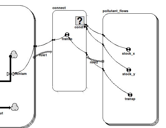
These names are recognized by Simile when the model is built, and the submodel properties are automatically edited to make it a multi-instance submodel with an instance for each flow connected to a compartment whose equation is at_posn(pollutant). 'stock_y' gets the row indices in the grid containing 'pollutant' for the positions of these compartments, either from their actual locations in their submodel or from the 2nd argument of at_posn() if present, while 'stock_x' similarly gets the column indices. 'transp' gets the values of the flows themselves (negated if they go out of the compartment concerned). The modeller may do anything she wants with these values, but the intention is to use them to set up a flow to the compartment in the grid submodel. This is most simply done by creating an association submodel between the grid and the submodel picking up the flow values (called 'connect' in the diagram). Here, 'transp' and the new flow 'contam' have the values 'role2_transp' and sum({'transp_role1'}) respectively, to simply pass the values between instances according to the relation. 'role1' has 'Allow base instance
lookup' selected in order to use one-sided relation enumeration to set up the relationship as efficiently as possible, not that this matters with only a handful of flows, and to do this the equation for cond1 must be 'index(2) is role2_stock_y and index(1) is role2_stock_x'
There will now be an instance of 'connect' relating each flow in the network model to the grid model instance where it takes effect. This image shows the grid helper displaying pollution hotspots resulting from the flows in the first image (note the correspondance between the positions of the pollution hotspots and the positions of the compartments within the map submodel in that image).
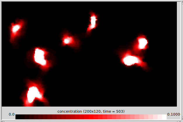
If your network model has squirts instead of, or as well as, flows that must affect the grid model, you should add another specially-named submodel to handle them, and interface that to the grid submodel as described above. The differences are as follows:
- its name should be target_squirts rather than target_flows (target is 'pollutant' in the example)
- the 'transp' component inside it is a derived event rather than a variable, which will occur when the corresponding squirt does
- the derived event in the relation model and the squirt in the grid model have the equation 'trigger_magnitude()'
- The influences connecting them have their properties set up so as only to include source events corresponding to the roles of the relation.
In: Contents >> Working with submodels