Built-in functions : Model properties

Model properties

Built-in functions : after function

after function

after(T, M)

Use only as whole equation of derived event. Instead of firing immediately when triggered, event is delayed by value of 1st argument, then fires with magnitude the 2nd argument had when triggered.

Inputs: Real, Any data type

Result: Same type as 2nd arg

In: Contents >> Working with equations >> Functions >> Built-in functions

Built-in functions : last function

last function

last(X)

Recalls value of X, another element, from previous time step. X must influence this element in order to be used in the equation. See prev, for a function that returns a previous value from this element itself.

This function has been replaced with the const_delay( ) and var_delay( ) functions, which are more general in allowing the value of a variable to be returned from an arbitrary number of time steps before.

Input: numeric

Result: numeric

In: Contents >> Working with equations >> Functions >> Built-in functions

Built-in functions : as_number function

as_number function

as_number(N)

Converts integral types to integer

Input: Boolean, enumerated type or integer (for flexibility)

Result: Value of argument as integer

In: Contents >> Working with equations >> Functions >> Built-in functions

Built-in functions : prev function

prev function

prev(N)

Returns the value of this element itself, N time steps ago. See last, for a function that returns a previous value of any element other than this one itself.

Input: numeric

Result: numeric

Example:

Consider a variable that flips from state 1 to state 2 when some triggering condition is satisfied (the Boolean variable, trigger, is true, for example) then stays in state 2. The equation for the variable could make use of prev, as follows:

if time()==0 then 1 elseif trigger then 2 else prev(1)

In: Contents >> Working with equations >> Functions >> Built-in functions

Built-in functions : parent function

parent function

parent(1)

Returns the id (instance number) of the individual whose reproduction gave rise to this one, or 0 if the individual being considered was created at the start of the simulation or by immigration.

Input: numeric (but a dummy value: use the value 1).

Result: integer (in fact, a negative integer number, being the instance number of a member of a population submodel. These are all numbered from -1 downwards.)

Comment:

This function is vital for the simulation of any form of biological inheritance from one generation to the next. You have to know who the parent is before you can allow the newly-created individual to inherit (possibly with modification) one or more of the characteristics of the parent.

In: Contents >> Working with equations >> Functions >> Built-in functions

Built-in functions : time function

time function

time()

Returns the current simulation time.

Input: none

Result: numeric (units = day)

Comment:

Any model which has exogenous variables (variables that change as a function of time, independently of the behaviour of the model, such as air temperature or rainfall) needs some way of knowing what the current clock time is: i.e. how far the simulation has proceeded. This function provides that information.

This function is not strictly-speaking necessary: you could get exactly the same behaviour by having a single compartment, initialised to zero, with a single flow in, with a constant value of 1. So, after 1 time unit the value of the compartment would be 1, after 12.5 it would be 12.5, and so on. However, the function is provided to avoid cluttering up the model with an extra compartment and flow.

In: Contents >> Working with equations >> Functions >> Built-in functions

Built-in functions : delay1, delay3, delayn functions

delay1, delay3, delayn functions

delay1(input, duration [, initial])

delay3(input, duration [, initial])

delayn(input, duration, n [, initial])

Arguments:

input: the value to be delayed

duration: time by which to delay the input value

n (delayn only): order of the material delay (delayn only)

initial (optional): the value of the result when the function first applies

Result:

The delayed value of input.

The delay1, delay3 and delayn function calculates a first, third or nth-order material delay of input, using an exponential delay time of delay duration, and an optional initial value initial for the delay. delay3 does this by setting up a cascade of three first-order material delays, each with a delay duration of delay duration/3. Other versions of the function behave analogously. delay3 returns the value of the final delay in the cascade. If you do not specify an initial value initial, all functions assume the value to be the initial value of input.

The delay3 function will return the value of delay 3 in the structure and equations shown in the following figure:

Compartment comp1 :
   Initial value = start_fill (real)
Compartment comp2 :
   Initial value = start_fill (real)
Compartment comp3 :
   Initial value = start_fill (real)
Flow delay 1 :
   delay 1 =        comp1*3/duration (1/day)
Flow delay 2 :
   delay 2 =        comp2*3/duration (1/day)
Flow delay 3 :
   delay 3 =        comp3*3/duration (1/day)
Flow inflow :
   inflow =        input (1/day)
Variable start fill :

start fill = initial*duration/3 (real)

Example:

Delay 3 = delay3(input, 5) where input = 5 + step(10,3) produces the pattern shown below:

Built-in functions : first function

first function

first(T)

Takes an argument T that is a member of an enumerated type, and returns "true" if it is the first member of its type, and "false" otherwise.

Input: enumerated type member, or array of enumerated type members

Result: boolean, or array of boolean values

Examples:

If enumerated type "fruit" is defined as "apple", "grape", "banana":

first("apple") --> "true"

first(["banana", "apple", "banana"]) --> ["false", "true", "false"]

In: Contents >> Working with equations >> Functions >> Built-in functions

Built-in functions : following function

following function

following(T)

Takes an argument T that is a member of an enumerated type, and returns the next member of the enumerated type.

Input: enumerated type member, or array of enumerated type members

Result: enumerated type member, or array of enumerated type members

Examples:

If enumerated type "fruit" is defined as "apple", "grape", "banana":

following("apple") --> "grape"

following(["grape", "apple", "grape"]) --> ["banana", "grape", "banana"]

In: Contents >> Working with equations >> Functions >> Built-in functions

Built-in functions : forcst function

forcst(<input>,<time>,<horizon>[,<initial>])

New in v6.6

The forcst function performs simple trend extrapolation. Here's how it works. First, forcst calculates the trend in input, based upon the value of input, the first order exponential average of input, and the averaging time. (Think of the averaging time as the time over which you wish to calculate a trend.) Then forcst extrapolates the trend into the future - you specify the distance into the future by providing a value for horizon. If you do not specify initial, forcst substitutes 0 for the initial value of the trend in input.

The forcst function is equivalent to the structural diagram and equations shown in this figure:

Put diagram here

Compartment Average input :

   Initial value = input-(averaging*initial) (real)
Flow change in average :
   change in average =        (input-Average_input)/averaging (1/day)
Variable averaging :
   averaging =        Variable parameter (day)
Variable forecast :
   forecast =        input*(1+trend*horizon) (real)
Variable horizon :
   horizon =        Variable parameter (day)
Variable initial :
   initial =        Variable parameter (real)
Variable input :
   input =        Variable parameter (real)
Variable trend :
   trend =        (input-Average_input)/(Average_input*averaging) (1/day)

Example:

Sales_Forecast = FORCST(Sales,10,15,0) produces a forecast of sales 15 time units into the future. The forecast is based on current sales, and the trend in sales over the last 10 time units. The initial growth trend in sales is set to 0.

Built-in functions : in_preceding function

in_preceding function -- new in Simile v5.7

Usage: in_preceding(expression of any type) returns that type

Definition: Used in a multi-instance submodel, returns the value of the argument expression as it would be in the preceding instance of that submodel, or 0 or "false" in the first instance. The argument can include the function prev(0) to refer to the value in the previous submodel instance of the component in whose equation the in_preceding() function appears.

Note that a model that contains a circular set of influences can build and run properly if the input parameter associated with one of the influences is only used in the argument of an in_preceding() function. This is because since the value of the argument is calculated for one submodel instance and then used in the next, there is no actual circular dependency.

Example 1:

A 5-instance submodel contains a variable with the equation

index(1)+in_preceding(prev(0)).

The values will be:

1 3 6 10 15

Example 2:

An 8-instance submodel contains two variables, "received" and "forwarded". These are connected to one another by influences in each direction. The equation for "forwarded" is received/2. The equation for "received" is

if index(1)==1 then 200 else in_preceding(forwarded)

The values of "received" for the 8 instances will be:

200 100 50 25 12.5 6.25 3.125 1.5625
In: Contents >> Working with equations >> Functions >> Built-in functions

Built-in functions : ramp function

ramp(time,slope)

Generates a ramp of slope slope, starting at time time and zero before that time.

Result: the ramp function.

Arguments: time at which to start ramping, slope (positive or negative) of ramp

Example:

the function ramp(20,-7) will have a return value of 0 at time 20 and -70 at time 30

Built-in functions : smth1, smth3, smthn functions

smth1, smth3, smthn functions

smth1(input, averaging [, initial])

smth3(input, averaging [, initial])

smthn(input, averaging, n [, initial])

Arguments:

input: the value to be smoothed

averaging: time over which to smooth the input value

n (smthn only): order of the material smoothing

initial (optional): the value of the result when the function first applies

Result:

The smoothed value of input.

The smth1, smth3 and smthn functions perform a first-, third- and nth-order respectively exponential smooth of input, using an exponential averaging time of averaging, and an optional initial value initial for the smooth. smth3 does this by setting up a cascade of three first-order exponential smooths, each with an averaging time of averaging/3. The other functions behave analogously. They return the value of the final smooth in the cascade. If you do not specify an initial value initial, they assume the value to be the initial value of input.

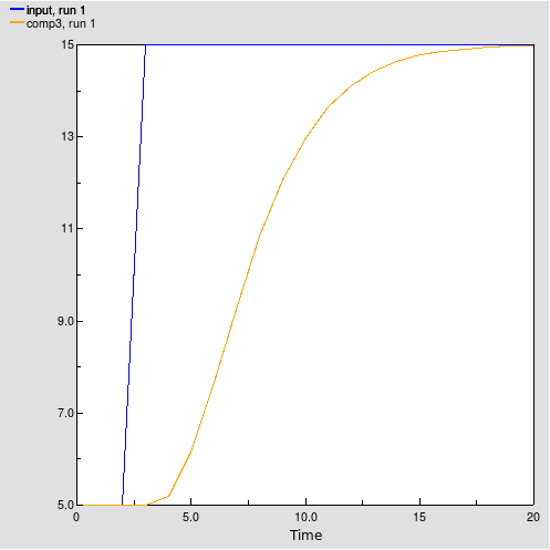
The smth3 function will return the value of comp3 in the structure and equations shown below.

Compartment comp1 :
Initial value = initial (real)

Compartment comp2 :
Initial value = initial (real)

Compartment comp3 :
Initial value = initial (real)

Flow flow1 :
flow1 = (input-comp1)*3/averaging (1/day)

Flow flow2 :
flow2 = (comp1-comp2)*3/averaging (1/day)

Flow flow3 :
flow3 = (comp2-comp3)*3/averaging (1/day)

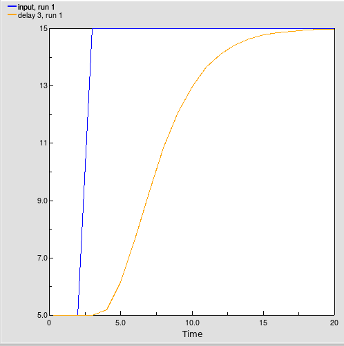
Examples:

Smooth_of_Step = smth3(Step_Input,5)

where

Step_Input = 5 + step(10,3) produces the pattern shown below.

Built-in functions : step function

step(height,time)

creates a step function. Output is 0 up until time, and equal to step thereafter.

Result: the step function.

Arguments: height of step, time at which to step.

Example:

step(30, 20) has output 0 at time 19, and 30 at time 20 and after

Built-in functions : stop function

stop function

stop(n)

Input: is a number (real or integer) of your choice

Result: None (see text)

When executed, this function halts execution of the model, and produces the following error message:

Simile ran into a problem trying to run this model.

While it was trying to calculate the value of variable

var (node x) during execution of the model at

time t, there was a user-defined interruption: n.

It is useful to define error conditions where you (the model designer) know that the model should not be used or is not applicable for some reason. Trivially, it can be used to guard against mathematical errors, for example:

if (time()-50) != 0 then 1/(time()-50) else stop(5)

This form has some merit when running in C++, but generally, to track down mathematical errors, it is easier to debug in Tcl. If execution in Tcl would take too long, then this is a useful alternative. Its primary use however, is to enable you to catch out-of-range conditions in the specific circumstances of your model.

The use of an error code in the user-defined interruption (e.g. stop(13) ) enables you to see which stop( ) function caused the model to stop running, if there is more than one in your model.

Result is undefined, because simulation stops at the point at which the function is called, but has integer type (this is important because if it is called in a conditional, the other branch of the conditional must also have a numerical type).

Examples:

if population>50 then stop(1) else 0

if (time()-50) != 0 then 1/(time()-50) else stop(5)

In: Contents >> Working with equations >> Functions >> Built-in functions

Built-in functions : trend function

trend(<input>,<time>[,<initial>])

New in v6.6

The trend function calculates the trend in input, based upon the value of input, the first order exponential average of input, and the exponential averaging time averaging time. trend is expressed as the fractional change in input per unit time. If you do not specify initial, trend substitutes the value 0 for the initial value of the trend.

The trend function is equivalent to the structural diagram and equations shown in this figure:

Put diagram here

Compartment Average input :

   Initial value = input-(averaging*initial) (real)
Flow change in average :
   change in average =        (input-Average_input)/averaging (1/day)
Variable averaging :
   averaging =        Variable parameter (day)
Variable initial :
   initial =        Variable parameter (real)
Variable input :
   input =        Variable parameter (real)
Variable trend :
   trend =        (input-Average_input)/(Average_input*averaging) (1/day)

Example:

Yearly_Change_in_GNP = TREND(GNP,1,.04)

This equation calculates the annual change in the input GNP. It starts with an initial value of .04 (4% per year).

Built-in functions : var_delay function

var_delay function

var_delay(var,n)

Input: a variable name and a numerical value (real or integer) of time units

Result: the value (any type) of the named variable, n time units ago

This function returns some previous value of another variable, an arbitrary period of time before. The period of time is defined in time units (not steps). The number need not be an integer, but whatever the actual time step, delay is always rounded to the nearest multiple of 0.1 of a time unit. The variable whose previous value is required is specified by name. The variables must be linked with an influence arrow.

This is a general replacement for the last( ) function, which returns the value of the named variable from the previous time step only. The delay must be between 0 and 100 and is rounded to the nearest 0.1. The delay can vary; if the delay is constant, the function const_delay() will do the job more efficiently.

Examples:

runoff=var_delay(rain,soak_time)

In: Contents >> Working with equations >> Functions >> Built-in functions

Built-in functions: at_init function

at_init function

at_init(X)

Returns the value the argument had when first used, i.e., on model reset or when the submodel instance containing this equation was created.

at_init(X) creates an implicit intermediate result, which has the same dimensions as its argument. So if this result is implicitly replicated elsewhere in the equation, the same value will be used each time. See makearray for behaviour in explicit replication.

Input: Any data type

Result: Same type as input

In: Contents >> Working with equations >> Functions >> Built-in functions

Built-in functions: at_posn function

at_posn function

at_posn(C)

at_posn(C,Row,Col)

Must form the whole equation of a component. Sets the component's value to the value of a component in an instance of a 2-D submodel representing a grid. C is the caption of the component in the grid submodel, and Row and Col if present are the outer and inner indices of the source instance (i.e., grid square) from which to get the value. If Row and Col are not present, the grid is mapped onto the diagram of the submodel containing the target component and the source instance selected by the component's position in the submodel diagram.

Input: Any data type plus optionally two integers

Result: Same type as input

In: Contents >> Working with equations >> Functions >> Built-in functions

Built-in functions: const_delay function

const_delay function

const_delay(var,n)

Input: a variable name and a numerical constant (real or integer) of time units

Result: the value (any type) of the named variable, n time units ago

This function returns some previous value of another variable, a arbitrary period of time before. The period of time is defined in time units (not steps). The number need not be an integer, but whatever the actual time step, delay is always rounded to the nearest multiple of 0.1 of a time unit. The variable whose previous value is required is specified by name. The variables must be linked with an influence arrow.

This is a general replacement for the last( ) function, which returns the value of the named variable from the previous time step only. The delay must be a numeric constant; for variable delay see var_delay().

Examples:

runoff=const_delay(rain,10)

In: Contents >> Working with equations >> Functions >> Built-in functions

Built-in functions: dies_of function

dies_of function

dies_of(X)

Returns true if argument is the loss channel that will cause the individual to disappear at the end of the current time step.

Input: value from a loss channel in the local submodel

Result: boolean

In: Contents >> Working with equations >> Functions >> Built-in functions

Built-in functions: in_progenitor function

in_progenitor function -- new in Simile v5.8

Usage: in_progenitor(expression of any type) returns that type

Definition: Used in a population submodel, returns the value of the argument expression as it would be in the instance of that submodel containing the reproduction channel responsible for the instance being evaluated, or 0 or "false" in an instance that arrived via a channel other than reproduction. The argument can include the function prev(0) to refer to the value in the progenitor submodel instance of the component in whose equation the in_progenitor() function appears.

Note that a model that contains a circular set of influences can build and run properly if the input parameter associated with one of the influences is only used in the argument of an in_progenitor() function. This is because since the value of the argument is calculated for the progenitor instance and then used in the offspring instance, and the progenitor always comes before the offspring in evaluation order, there is no actual circular dependency.

Important: If the progenitor instance has been removed (see Extermination) then using this function will return meaningless values, and may cause model execution to be aborted due to memory access violations. To avoid this problem, make the in_progenitor function itself the argument of an at_init() function, e.g., at_init(in_progenitor(index(1))). If this is done, the inner argument will be evaluated for the progenitor instance when the offspring instance is created -- at which time the progenitor definitiely exists -- and then retained within the offspring instance's data structure. The only reason for not doing this would be if changes in the value in the progenitor continue to affect the offspring, and offspring never outlive their progenitors, e.g., in an L-systems model of tree branching.

In: Contents >> Working with equations >> Functions >> Built-in functions

Built-in functions: iterations function

iterations function

iterations(X)

Returns number of iterations that have been done up to this point in an alarm submodel. Argument is the boolean balue from the alarm symbol.

Input: value from an alarm symbol in the local submodel

Result: integer

In: Contents >> Working with equations >> Functions >> Built-in functions

Built-in functions: preceding function

preceding function

preceding(T)

Takes an argument T that is a member of an enumerated type, and returns the previous member of the enumerated type.

Input: enumerated type member, or array of enumerated type members

Result: enumerated type member, or array of enumerated type members

Examples:

If enumerated type "fruit" is defined as "apple", "grape", "banana":

preceding("grape") --> "apple"

preceding(["banana", "grape", "banana"]) --> ["grape", "apple", "grape"]

In: Contents >> Working with equations >> Functions >> Built-in functions

Built-in functions: pulse function

New in v6.6. Note this function is provided purely for compatibility with continuous-only modelling tools, and new models should use squirts instead.

pulse function:

pulse(magnitude, first_time [, interval])

Generate a pulse with a duration of a single time step and a given cumulative value.

Result: the pulse waveform

Arguments:

magnitude: the cumulative value of the pulse. This will be the level change of a compartment due to a flow with this value coming into it.

first_time: The first, last or only time at which the pulse will occur

interval (optional) : If this is positive, the pulse will occur regularly with this interval after the initial time

If it is negative, the pulse will occur with this interval up until the initial time and not after

If zero or not present, the pulse will occur only once at the initial time

Example: pulse(20, 12, 5) generates a pulse value of 20/DT at time 12, 17, 22, etc.

Built-in functions: trigger_magnitude function

trigger_magnitude function

trigger_magnitude()

Returns a value representing the magnitude of the triggering event. Can only be used in the equations of derived events, squirts and rule-based state variables. Events influencing these components are not listed as parameters so this function is used to get their values. If the trigger is a simple event, this function gives the value of that event's equation. If it is a time series, it is the current value from the series. If it is a limit event then it is 'true' if there is only one limit, and -1/1 for lower/upper limit if both are given.

Inputs: none

Result: same units and dimensions as triggering events

In: Contents >> Working with equations >> Functions >> Built-in functions

Built-in functions : sofar function

sofar function

sofar([X])

sofar({X})

Result is…

Input: numeric array/list

Result: numeric

Example:

Comment:

In: Contents >> Working with equations >> Functions >> Built-in functions

Built-in functions : size function

size function

size(S)

size(S,I)

The first form takes the name of a fixed-membership submodel and returns the number of instances that it has. The second form takes the name of a fixed-membership submodel and returns the size of the Ith level of nesting of this submodel.

Input: submodel name

Result: integer

In: Contents >> Working with equations >> Functions >> Built-in functions

Built-in functions : dt function

dt function

dt(I)

Returns the duration of the level I time step.

Input: numeric. This is the time step level.

Result: numeric

Examples:

dt(1) --> 0.1 (for a model whose top-level time step was set to 0.1 in the Run Control panel)

dt(2) --> 0.001 (for a model whose 2nd-level time step was set to 0.001 in the Run Control panel)

If you are starting off with Simile, it is unlikely you will need to understand the concept of "time step index". You will probably just be making models with a single time step, hence one level, so don't worry about anything except the use of dt(1).

The main use of the dt function is to engineer the addition or removal of a specified amount of a substance into or out of a compartment. The only handle we have for causing changes to the amount in a compartment are flows, and flows are expressed as a rate per unit of time (whatever time unit is used for the model, e.g. year). This creates a problem if we want to add or remove a specified amount of substance at some instant in time. For example, consider a model with a time unit of year, a time step of 0.1, and with a compartment X from which we want to remove 5 units at the instant that some condition, which only lasts for 1 time step (0.1 years), is met. If we simply had a flow out that was zero when the condition was not met, and was 5 when the condition was met, then for one time step the flow would be 5 (units per year): hence, only 0.5 units would be removed in the 1/10th of a year, not the 5 we intended. What we need to do is to artificially inflate the flow rate by a factor of 10 (in this case, with a time step of 0.1) for this one time step. We do this by dividing the flow rate (in our flow equation) by 0.1 (in this case), or by dt(1) in general. The flow rate then appears to be 50 units per year for that one time step, giving a loss of 5 units in the one time step. Bingo!

The actual flow expression for the case considered above would be:

flowout = 5/dt(1)

Special case

Using the argument zero in the function, i.e. dt(0), is equivalent to saying dt(n), where n is the time step index of the submodel in which the function is used. This is useful, because when a submodel time step index is changed, it is then not necessary to edit the dt() functions within it to preserve the meaning.

In: Contents >> Working with equations >> Functions >> Built-in functions

Built-in functions : count function

count function

count([X])

count({X})

Number of values in the array [X] or the list {X}

Input: array or list of values (numeric or boolean)

Result: integer

Examples:

count([4,5,6]) --> 3

In: Contents >> Working with equations >> Functions >> Built-in functions

Built-in functions : channel_is function

channel function

channel_is(X)

X is an immigration, reproduction or creation channel. Returns true if this individual appeared through that channel.

Input: numeric

Result: Boolean

Examples:

channel_is(cr1) --> true, for each instance of the population that was initially created through channel cr1.

Comments:

This function can only be used inside population submodels. Its argument is the name of a channel (i.e. a population control symbol, one of creation, immigration or reproduction). Note that the value of the channel itself is not used, just the name. The result can be used in calculations inside the population submodel. For example, the expression

land_owned = if channel_is(im1) then 0 elseif channel_is(cr1) then 10

would allocate 10 acres of land to each member of the original population, but none to immigrants.

In: Contents >> Working with equations >> Functions >> Built-in functions

Built-in functions : init_time function

init_time function

init_time(1)

Returns the time at which this model component first came into existence. This really only has any use for:

population submodels, so that the model knows when a new member of the population was created; and
conditional submodels, so that the model knows when the submodel, or one instance of it, came into existence because the condition controlling it became true.

Input: numeric. In fact, the argument is not used, so simply insert the number 1. The only reason for having the brackets and an argument enclosed between them is that this is the only way that Simile can recognise that this is a function.

Result: numeric

Example:

Let's assume you have a population submodel, and some property of each individual is related to its age (e.g. its growth rate, or its probability of dying). Simply create a variable called age (inside the submodel), and insert the following equation:

age = time(1) - init_time(1)

The result is the difference between the current simulation time (given by the function time(1), and the time when the instance was created, given by init_time(1).

In: Contents >> Working with equations >> Functions >> Built-in functions

Built-in functions : index function

index function

index(I)

Returns the index (instance number) of a member of a fixed membership or population submodel, for the level of submodel nesting specified by the argument.

Input: numeric

Result: numeric

Comment:

The index function is frequently used in conjunction with the element function when working with multiple-instance submodels: both fixed-membership and population submodels.

The argument specifies which index is to be returned. You can see summary information about the meanings of the different indices in the listbox headed Indices: in the equation dialogue. The argument is an integer between 1 and the maximum number of indices available. index(1) corresponds to the 'innermost' index, i.e., if you have one multiple-instance model inside another, the result of index(1) will be the index of the inner submodel instance, and the result of index(2) will be that of the outer submodel instance. Similarly, if a submodel has two dimensions, then index(1) and index(2) will be valid in that submodel, giving an instance's position along the inner and outer dimension respectively.

Relation submodels do not usually have indices of their own, but you can get the indices of their base submodel instances using the index() function. If one of the roles in a relation has been specified to 'allow base instance lookup', then the base submodel for this role will be 'innermost' and and the index of the instance in this role will be the result of calling 'index(1)' in the relation submodel.

For fixed-membership submodels, the function returns an integer value between 1 and n, where n is the number of instances for the submodel. For variable-membership submodels, it returns an integer between 1 and n, where n is the maximum possible index. For a population submodel this would be the total number of instances of the population that have ever existed during this simulation run. For a conditional submodel the maximum will be the size given in the submodel dimensions. For either of these, an instance with a particular index number may or may not exist.

In: Contents >> Working with equations >> Functions >> Built-in functions