Model Gallery
You can use this page to get a quick overview of the wide range of models that can be constructed in Simile. Each entry gives some text on the model, a model diagram (usually an outline view for all but the simplest of models), and a sample screen display from the running model. Models are arranged roughly in order of increasing complexity and increasing sophistication of the Simile techniques used.
Classic (Lotka-Volterra) population dynamics
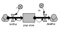
Exponential population growth
The population is represented by a single state variable (compartment), whose dynamics depends on two flows: a reproduction inflow and a mortality outflow. Both occur at a rate proportional to population size, where r and m are the coefficients of proportionality.
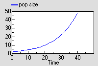
The graph shows the expected exponential increase in population size.
Logistic (sigmoid, density-dependent) population growth
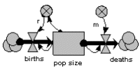
The previous model is modified by making r, the reproductive rate per individual, depend on population size, decreasing as population increases.
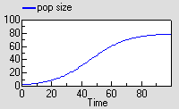
This causes the population to grow roughly exponentially to begin with, but then rise more slowly towards a “carrying capacity”.
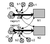
Two-species competition
Each population grows logistically in the absence of competition, with its growth rate reduced as its population gets bigger. When a competitor is present, then the growth of each population is further reduced by the other. The outcome depends on the relative strength of within- and between-species factors.
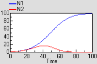
The graph shows that both species initially grow at similar rates, but then species 1 escapes and suppresses species 2.
Predator – prey
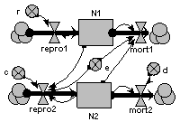
The prey (N1) grows exponentially in the absence of predation. It is predated at a rate proportional to the number of predators. The growth rate of the predator propulation is proportional to prey consumption, and predator mortality is proportional to its population.
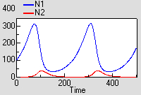
This model shows the classic (but rather mythical) predator-prey cycle.
Model gallery : age-class disaggregation
Population age-class models
Explicit compartments
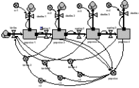
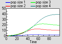
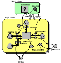
The simplest way of making an age-class model is to have a separate compartment for the number in each class. The compartments are connected by flows representing the movement of animals between classes as they age. Reproduction feeds into the first class, and all classes have a mortality outflow. This particular model includes density-dependent reproduction.
The model eventually equilibrates with a fixed number in each class.
Multiple-instance submodel
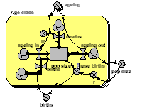
In this model, each age-class is now one instance of a fixed-membership, multiple-instance submodel. It has a compartment (the number in that each class), and associated flows. Outside the submodel we have an array for transferring those leaving one class to the next class, an array for the births from each class, and a variable for total population size.
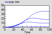
Running the model produces exactly the same results as for the previous model, though this time the results are shown for each instance of one variable.
Multiple-instance submodel with an association between classes
Again, a multiple-instance fixed-membership submodel is used to represent each age-class. But in this model the transfer of individuals from one class to the next takes place through an association submodel, defined in terms of the relationship between one class and the next. This is a more expressive, flexible and (for complex models) more efficient way of linking classes.
The results are excatly the same as for the previous model.

Model gallery : individual-based disaggregation
Individual-based model of population dynamics
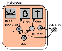
This shows how amazingly simple it is to make an individual-based model of population dynamics in Simile. We simply create a population submodel, add in symbols for the initial number, birth and death. In this model, the probabilities of reproduction and death are age-dependent, and reproduction also depends on the total population size, which is simply obtained by summing the number of individuals.
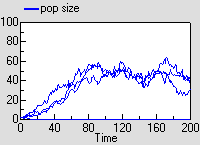
Since this is a stochastic model, each run is different. The graph shows the result of three runs., showing the population increasing and hovering around an equilibrium.
Model gallery : custom display tools
Individual-based tree model
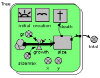
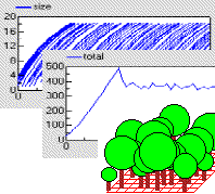
This model uses a population submodel to represent the trees in a forest stand. A simple, single-compartment model is used to simulate the growth of each tree, and this is summed outside the submodel to give the total volume of the stand of trees. The model also sets the initial number of trees in the population, the rate at which new trees are created, and the rule for killing off trees when they reach a certain size.
The graphs show the growth of each tree, from birth to death, and the volume of the whole stand. The custom “lollipop diagram” represents the stand structure during the simulation, using the tree’s (x,y) coordinates to position the trees.
Model gallery : fractals
Fractal model of tree branching
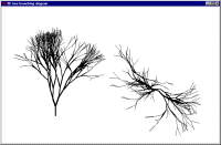
Fractal branching models - frequently called Lindemeyer or L-system models - work by repeated application of the same branching rules. The Simile implementation uses a population submodel for the branch segments (intenodes), starting off with a single member (the base segment). An association submodel is used to define the relationship between one segment and its two daughters.
The behaviour of the model is visualised using a specially-developed display tool, showing the 3D structure of the simulated tree from the side and from the top.

Model gallery : animation
Animal movement model
We represent a number of animals using a fixed-membership multiple-instance submodel (it is easy to make it into a population submodel, if you wanted a dynamically-varying population). Each animal has got three state variables, representing its current x,y coordinates and the direction it’s going. Its direction changes slightly from one time step to the next, and this, along with its speed is used to update its position. Each animal is constrained to stay within the area.
We can visualise the animals’ movement using any display tool that can plot x,y values: here I've used the lollipop helper, in plane projection.


Model gallery : spatial associations
Multi-layer soil water model
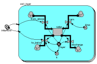
This example shows the use of a fixed-membership multiple-instance submodel for modelling the movement of water through soil layers. Each instance represents one layer, and has a single compartment, for the amount of water in that layer. The array variable outside the submodel is used to transfer the water flowing out of one layer into the one below it.
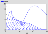
The graph shows the behaviour of the model in response to a pulse of rain lasting 8 hours. The top layer responds quickly, followed by the ones below it. The bottom layer has a lower discharge rate.
Model Gallery: where next?
For a more in depth look at some models have a look at the worked examples and a wide range of models with varying quality of documentation can be found in the model catalogue.