5. Using a population submodel
The above examples all share one thing in common: they represent a population in terms of the values for one or more state variables, there being as many state variables as there are classes in the population. Each state variable may be engineered to have integer values (on the basis that populations contain a discrete number of individuals), or to have real (floating point) values, if you are content to think in terms of population density (i.e. number per unit area) rather than absolute numbers. The number of state variables (hence the computational requirement) is fixed, and totally independent of the number of individuals in the population.
A totally different approach is to represent each individual in the population separately. This can be justified on the basis of what is considered necessary to adequately capture the factors driving population dynamics. For example, if we know that social interactions between individuals is important, then we need some way of capturing these: it may be difficult to approximate to their effects in a lumped or class-disaggregated model.
Since we are interested in population dynamics, building an individual-base model will require that we create new individuals as time goes on, and remove existing ones. Thus, the amount of memory required to manage this population will change as the simulation proceeds. If the model is implemented by programming, the difficulty of doing this increases substantially as we move from a fixed number of state variables to a dynamically-changing list.
In Simile, it is very easy to create an individual-based model. You simply use a Simile submodel to define how one individual works, then declare this submodel to be a population submodel. You can then add model elements to hold the equations or rules for the creation of new individuals and the killing off of existing ones.
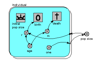
Here’s a model which is the individual-based equivalent of the age-class model with density-dependent reproduction. We make a submodel and call it “Individual” (following the principle that the label for a multiple-instance submodel should reflect the single object it references). It is specified as a population submodel by simply choosing this option in the submodel properties box. A population submodel is drawn with shadow lines on the top-left and bottom-right, to distinguish it from the fixed-membership multiple instance submodel we have seen so far.

It has symbols for representing the initial number (i.e the number created when the model is initialised), an expression for creating new individuals by reproduction of existing ones (“birth”), and an expression for deciding when an individual dies (“death”). For consistency with the notation of the earlier models, we have two parameters, r and m, with similar meaning as before: r represents the probability that an individual will reproduce in one unit of time, and m represents the probability that an individual will die. Both r and m depend on the individual’s age (calculated simply as the difference between the current simulation time and the time when the individual was created). r also depends on the size of the population (negative density dependence). The population size is calculated as the sum of the value 1 (held in the variable “one”) over all the individuals. Note that population size has to be outside the individual submodel, since it is an attribute of the whole population, not of any one individual.
This model is now a stochastic one: the parameters r and m are treated as probabilities rather than deterministically generating changes to the population. We could have handled these deterministically - for example, creating one new individual when we had accumulated sufficient credit — but a stochastic interpretation is more intuitive. We could also have made the previous models stochastic (by sampling from a distribution to get the annual reproductive inputs and mortality losses), but then we would have lost the link with standard textbook models of population dynamics.
You may be surprised to see that there are no compartments here. We could have them: for example, we may want to model the change in body weight of each individual (or, say, height of each tree), in which case we could have a compartment and associated flows inside the submodel. We could equally well choose to have a complex System Dynamics model if, for example, we have a sophisticated, physiologically-based model of tree growth and we want to model a stand of trees on that basis. But this example shows that we do not have to include compartments and flows in a Simile model. Nevertheless, we can still use part of System Dynamics notation: the variable and the influence arrow.
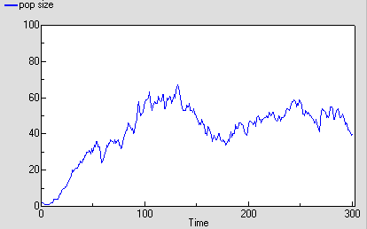
The following graph shows one run with the model. It’s run for 300 time units, since the reaching of an asymptote after 100 time units is less clearcut with this stochastic model. Even then, its stochastic nature means that there is considerable variation after reaching balance.

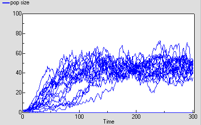
The following diagram shows the result for 25 replicate runs. The basic logistic growth can be discerned. It is also clear that the stochastic nature is more than simply variation around this line: some runs take quite a while to take off, and in fact in some cases the population goes extinct.
