Working with equations : Functions

Functions

Simile provides a large number of built-in functions that can be used in mathematical expressions. These include standard mathematical functions, such as log(…) as well as functions specific to Simile.

Some functions have one or more arguments (in brackets, after the function name). Others, such as the time() function, which returns the current simulation time, do not. You must still write the brackets after the function name, even if there are no arguments. This indicates that the name is a function name.

For most functions, the arguments are scalar values, i.e. a single quantitative value. In some cases, an argument is expected to be some other type of data structure, such as a Boolean value (true or false), or an array or list (such as the sum(…) function, which returns the sum of the values in an array or list.


It is possible to include user-defined functions. These can be specific to modelling in a restricted domain (such as plant physiology), so it will be possible for researchers in a particular community to build up and share common libraries of functions. 

Two special functions are graph(…) and table(…), which relate to a graphically-represented and a tabulated relationship respectively. These can be included in an expression like any other function, but differ from other functions in that the result they return for a given input value can be different in each equation in which it is used: it's definition is local to the equation, rather than being universally defined (like the log(…) function, for example).

In: Contents >> Working with equations >> Components of an equation

Working with equations : Built-in functions

Built-in functions

Alphabetical list of most commonly used functions,  Trigonometric functions are listed separately. Please see the other categories at the bottom of the page for less common or recently added functions.

 Template  Effect

Input(s)

Return

value

abs(X)

Returns the absolute value of X


all([X])

all{X})

Result is true if all the elements of the array [X] or the list {X} are true

boolean array/list

 Boolean

any([X])

any({X})

Result is true if any of the elements of the array [X] or the list {X} are true.

boolean array or list

 Boolean
at_init(X) Returns X's value when last initialized or reset Any Same as input

at_posn(C)

at_posn(C, X, Y)

Causes component to get value from instance of C in a grid submodel Any, two optional integers Scalar as 1st argument
binome(P, N) Returns a value from the binomial distribution with probability P and number of trials N

Real value from 0 to 1,                  Integer value

Integer value

ceil(X)

Rounds up X to the next whole number


channel_is(X)

X is an immigration, reproduction or creation channel. Returns true if this individual appeared through that channel.

   
colin([X]) Returns an index to the given array, with probabilities proportional to the array's values Array of numeric values Integer or enumerated type member
const_delay(X, T) Returns the value of X as it was T time units earlier in the run, or 0 or "false" if the component did not exist at that time Any non-array type, numeric constant As 1st argument

count([X])

Number of values in the array [X] or the list {X}

scalar array/list


delay1(x,t), delay3(x,t), delayn(x,t,n)

Insert a material delay of order 1, 3 or n

numerical

numerical, numerical, integer (delayn only)
dies_of(X) X is a loss channel. True if channel specifies the removal of the individual this time step. from loss channel Boolean

dt(I)

Returns the duration of the time step level I


element([X],I)

Picks the I'th value form the array [X]

array of any type,integer or enumerated type member


exp(X)

Returns e to the power X


exprnd(mean [, seed])

Samples an exponential distribution

numerical[, integer] numerical
first(T) Returns "true" if argument is the first member of its enumerated type Enumerated type member Boolean
firsttrue([B]) Takes an array of booleans and returns the index of the first with value "true" Array of booleans Integer or enumerated type member

floor(X)

Rounds X down to a whole number


fmod(X,Y)

Returns remainder after dividing X by Y

numeric, numeric

 
following(T) Returns next member of argument's enumerated type Enumerated type member Enumerated type member
forcst(input, time, horizon [, initial]) New in v6.6: Performs simple trend extrapolation Real, real, real [,real] Real
gaussian_var(X,Y) Returns a sample from a Gauusian distribution with mean X and SD Y Real, real real

greatest([X])

greatest({X})

Returns the largest value from an array [X] or the list {X}

numeric array/list

 
howmanytrue([B]) Takes an array of booleans and returns the number that are true List or array of booleans Integer
hypergeom(P, M, S) Returns a deviate from a hypergeometric distribution for population, P, number of marks M, and sample size S. integer, integer, integer integer

hypot(X,Y)

Returns length of hypotenuse of triangle with base X and height Y

numeric, numeric


index(I)

Returns the index (instance number) of a member of a fixed membership or population submodel, for the level I of submodel nesting.

 Integer Integer or enumerated type member

inf()

New in v6.6: Returns the value of positive infinity.

 Real None

init_time(1)

Returns the time at which this instance appeared -- argument is dummy

   
in_preceding(X) New in Simile v5.7: Returns value of X in preceding submodel instance Any scalar or array type As argument
in_progenitor(X) New in Simile v5.8: Returns value of X in submodel instance that reproduced to make current one Any scalar or array type As argument

int(X)

Returns integer part of X

   
interpolate(X, [Xarray], [Yarray]) Returns interpolated value from [Yarray] corresponding to X's place in Xarray

Numeric, Array of numeric, Array of numeric

Numeric
iterations(B) Counts executions of iterative submodel Boolean Integer

last(X)

Recalls value of X from previous time step


least([X])

least({X})

Returns the smallest value from an array [X] or the list {X}

numeric array/list


log(X)

Returns natural logarithm of X


log10(X)

Returns base-10 logarithm of X


makearray(X,N)

Makes an array consisting of N lots of X

any type, integer

array of same type

max(X,Y)

Returns greater of X and Y

numeric, numeric


min(X,Y)

Returns lesser of X and Y

numeric, numeric

 
order([X]) Returns an array holding the indices of the argument array in ascending order of their values array of numeric array of integer

parent(I)

Returns the id of the individual whose reproduction gave rise to this one, or 0 if it immigrated or was created


place_in(I)

When making an array with makearray, this gives each term's position in the array -- argument is nesting depth

   
poidev(X) Returns a value from the Poisson distribution with the given mean numeric integer
posgreatest([X]) Returns the index of the highest value in the argument array Array of numeric values Integer or enumerated type member
posleast([X]) Returns the index of the lowest value in the argument array Array of numeric values Integer or enumerated type member

pow(X,Y)

Returns X raised to the power Y

numeric, numeric

 numeric
preceding(T) Returns previous member of argument's enumerated type Enumerated type member Enumerated type member

prev(N)

Returns the value of this component N time steps ago


product([X])

product({X})

Result is the product of all elements of the array [X] or the list {X}

numeric array/list

numeric

pulse(H, T [, I])

Generates a single time step pulse of magnitude M at time T, and before or after at intervals of I if I present

numeric, numeric, numeric

numeric

ramp(T,S)

Generate a linearly increasing or decreasing value over time with the given slope

numeric, numeric

numeric

rand_const(X,Y)

(Deprecated) Returns a random number between X and Y, which stays the same until the simulation is reset.

numeric, numeric


rand_var(X,Y)

Returns a random number between X and Y, with a new value every time step.

numeric, numeric

 
rankings([X]) Returns ranking of each element in order of size Array of numerics Array of integers

round(X)

Rounds X up or down to the nearest whole number

   
sgn(X) Returns the size of X; -1 if negative, 1 otherwise    

size(S)

Takes the name of a fixed-membership submodel and returns the number of instances that it has.


size(S,I)

Takes the name of a fixed-membership submodel and returns the size of one of its dimensions

submodel, numeric


smth1(x,a), smth3(x,a), smthn(x,a,n)

Insert a material smoothing of order 1, 3 or n

numerical

numerical, numerical, integer (smthn only)

sqrt(X)

Returns the square root of X


step(H, T)

Generate a step increase (or decrease) at the given time

numeric, numeric numeric

stop(X)

Stops the simulation, displaying value of X in a popup message

   
subtotals([X])

Returns running totals from summing the elements in the supplied array

Numeric array Numeric array

sum([X])

Result is the sum of all elements of the argument

numeric array/list


time()

Returns the current simulation time (the argument is ignored)

   
trigger_magnitude() Returns value of triggering event    As triggering event
var_delay(X,T) Returns value of X as it was T time units earlier in run, or 0 or "false" if this is before component existed Any non-array type, numeric expression As first argument

with_colin({N},{X})

Returns a value from the list {X} with probabilities proportional to the corresponding values in the list {N}

numeric list,       any list

member of second arg

with_greatest([N],[X])

with_greatest({N},{X})

Returns the value from an array [X] or the list {X} whose position in the array or list corresponds to the largest value in the array [N] or list {N}

numeric array/list, any array/list


with_least([N],[X])

with_least({N},{X})

Returns the value from an array [X] or the list {X} whose position in the array or list corresponds to the smallest value in the array [N] or list {N}

numeric array/list, any array/list


In addition, a full range of trigonometric functions are provided.

In: Contents >> Working with equations >> Functions

Built-in functions : Arithmetic functions

Arithmetic functions

Built-in functions : abs function


abs function

abs(X)

Returns the absolute value of X - i.e. ignores its sign

Input: numeric scalar or numeric array

Result: numeric scalar or array

Examples:

abs(3) --> 3

abs(-3) --> 3

abs([2,-3,4,-5]) --> [2,3,4,5]

In: Contents >> Working with equations >> Functions >> Built-in functions

Built-in functions : pow function


pow function

pow(X,Y)

Returns X raised to the power Y

Input: numeric, numeric

Result: numeric

Comment:

This is equivalent to the use of the ^ operator: i.e.

pow(5,2)

is the same as

5^2

The latter should be used of preference, as it is the more familiar notation.

In: Contents >> Working with equations >> Functions >> Built-in functions

Built-in functions : min function


min function

min(X,Y)

Returns lesser of X and Y; i.e. it returns X if X<=Y, otherwise it returns Y.

Inputs: numeric, numeric

Result: numeric

Comments:

The min function is a useful way of ensuring that some value does not go above some threshold. For example, if b increase as a increases, but does not exceed 20, then the equation for b could be:

b = min(20, 0.2*a)

This avoids the use of a cumbersome if…then… else… construction

In: Contents >> Working with equations >> Functions >> Built-in functions

Built-in functions : max function


max function

max(X,Y)

Returns greater of X and Y; i.e. it returns X if X>=Y, otherwise it returns Y.

Inputs: numeric, numeric

Result: numeric

Comments:

The max function is a useful way of ensuring that some value does not go below some threshold. For example, if b declines as a increases, but does not go below zero, then the equation for b could be:

b = max(0,10-0.2*a)

This avoids the use of a cumbersome if...then...else... construction.

In: Contents >> Working with equations >> Functions >> Built-in functions

Built-in functions : inf function

inf function

New in v6.6

inf()

Returns the value of positive infinity

Input: none

Result: numeric

Built-in functions : sgn function

sgn function

sgn(X)

Returns -1 if X is negative, or 1 if X is zero or positive

Input: numeric, or array of numeric values

Result: integer, or array of integer values

Examples:

sgn(1.9) --> 1

sgn(-1.1) --> -1

In: Contents >> Working with equations >> Functions >> Built-in functions

Built-in functions : sqrt function


sqrt function

sqrt(X)

Returns the square root of X

Input: numeric

Result: numeric

In: Contents >> Working with equations >> Functions >> Built-in functions

Built-in functions : round function


round function

round(X)

Rounds X up or down to the nearest whole number

Input: numeric, or array of numeric values

Result: numeric, or array of numeric value

Examples:

round(1.9) --> 2

round(1.1) --> 1

round([1,2.1,3.9]) --> [1,2,4]

In: Contents >> Working with equations >> Functions >> Built-in functions

Built-in functions : log10 function


log10 function

log10(X)

Returns base-10 logarithm of X

Input: numeric

Result: numeric

In: Contents >> Working with equations >> Functions >> Built-in functions

Built-in functions : log function


log function

log(X)

Returns natural logarithm of X

Input: numeric; or an array of numeric values

Result: numeric; or an array of numeric values

In: Contents >> Working with equations >> Functions >> Built-in functions

Built-in functions : ceil function


ceil function

ceil(X)

Rounds up X to the next whole number (stands for 'ceiling')

Input: numeric, or array of numeric values

Result: numeric, or array of numeric value

Examples:

ceil(1.9) --> 2

ceil(1.1) --> 2

ceil([1,2.1,3.9]) --> [1,3,4]

In: Contents >> Working with equations >> Functions >> Built-in functions

Built-in functions : exp function


exp function

exp(X)

Returns e (the base of natural logarithms) to the power X

Input: numeric, or an array of numeric values

Result: numeric, or an array of numeric values

Example:

The exponential growth of a population is given by the formula

Nt = N0er.t

where:

Nt is the population size at time t,

N0 is the initial population size,

e is the base of natural logarithms,

r is the intrinsic growth rate, and

t is current time
 

We can represent this in Simile using a single variable (called N), with its equation being

N = 10*exp(0.1*time(1))

assuming that the initial population size = 10 and the value of r is 0.1.
 

In: Contents >> Working with equations >> Functions >> Built-in functions

Built-in functions : floor function

floor function

floor(X)

Rounds X down to a whole number.

Input: numeric, or an array of numeric values

Result: numeric, or an array of numeric values

Examples:

floor(3.1) --> 3

floor(3.99) --> 3

floor([1.1,2.4,3.7,4.9]) --> [1,2,3,4]

In: Contents >> Working with equations >> Functions >> Built-in functions

Built-in functions : int function


int function

int(X)

Returns integer part of X

Input: numeric

Result: numeric

In: Contents >> Working with equations >> Functions >> Built-in functions

Built-in functions : hypot function


hypot function

hypot(X,Y)

Returns length of hypotenuse of right-angle triangle with base X and height Y

Inputs: numeric, numeric

Result: numeric

Examples:

hypot(3,4) --> 5 (a 3:4:5 triangle)

hypot(x1-x2,y1-y2) --> the distance between two points with co-ordinates (x1,y1) and (x2,y2) respectively.

hypot(x-[xs],y-[ys]) --> [distances] I.e. an array containing the distance from one point with co-ordinates (x,y) to a set of points, with co-ordinates held in the arrays [xs] and [ys]. See comments.

Spatial modelling frequently requires that one object knows the distance to another. This requires that each has x,y co-ordinates. It is then simple to use the hypot function to work out the straight-line distance between them, as shown in the second example above.

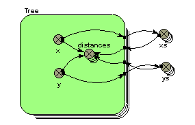
The same principle applies when you use a multiple-instance submodel to represent a set of spatially-located objects. In this case, each object may want to know how far it is to all the other objects - for example, in working out the competition between trees in an individual-based tree model. The following model diagram fragment shows a typical model configuration for doing this:

Each tree has x,y co-ordinates. These are exported to two array variables, xs and ys, whose equations are simply:

xs = [x]

and

ys = [ys]

These arrays are then brought back into the submodel, and used to generate an array containing the distance for each tree to all the other trees, using the equation given in the third example above.

In: Contents >> Working with equations >> Functions >> Built-in functions

Built-in functions : fmod function


fmod(X,Y)

Returns remainder after dividing X by Y

Inputs: numeric, numeric

Result: numeric

Examples:

fmod(7,3) --> 0.333 (7/2 = 2.333, i.e. the remainder is 0.333)

fmod(time(1),1) --> a result that climbs from 0 to 1 repeatedly (i.e. a sawtooth pattern) as the simulation proceeds. See comments below.

fmod((index(1)-1),5)+1 --> 1,2,3,4,5,1,2,3,4,5,1,2,3... for successive values of index(1). See comments below.

This apparently obscure function in fact has (at least) two very valuable uses.

First, it can be used to generate regular cycles, in particular annual or daily cycles. Consider the case or a model with the time unit being one year, and a time step of less than a year. You want various exogenous variables (such as temperature or rainfall) to vary in a prescribed fashion during the course of each year, with the annual pattern repeating itself from one year to the next. The following diagram is typical of the model fragment you could use for representing this:

The variable time is simply set equal to current simulation time, using the function time(1). The variable season is set to rise from 0 to 1 every year. If your model used a time unit of one week, then the equation would be changed to

season = fmod(time,52)

and the value for season would then correspond to week number. The equations for rainfall and temperature are for illustration purposes only: you would need to replace them by something appropriate.

Second, the fmod function can be used to generate a regular spatial arrangement (rows and columns) for a 2D grid. Let's say that you are modelling an area of 10x10 grid squares. In Simile, you would set up a submodel, called perhaps Patch, with 25 instances. In order to give each patch location on a grid, each one needs to have a row and column attributes, with each patch having a unique combination of the numbers 1..5 for row and column. The only thing we know about each patch is that it has an index number (given by the built-in function index(1)), a value ranging between 1 and 25. The trick is to get row number to be, in sequence,

1,1,1,1,1,2,2,2,2,2,3,3,3...

and column number to be, in sequence,

1,2,3,4,5,1,2,3,4,5,1,2,3...

thus giving each of the 25 instances a unique row-and-column pair.

This is readily done using the following two equations:

row = floor((index(1)-1)/5)+1

column = fmod((index(1)-1),5)+1

See the floor function to understand why the row numbers should be in the first sequence above. For column, we divide the index number for each instance by 5, taking the remainder: the '-1' and +1' are there to ensure that we get the results in the blocks of five that we require. See a grid-based spatial model example to see this in action.

In: Contents >> Working with equations >> Functions >> Built-in functions

Built-in functions : Trigonometric functions

Trigonometric functions


Input(s)


acos(X)

Returns the arccos (inverse cosine) of X. Result is in radians.


asin(X)

Returns the arcsine of X. Result is in radians.


atan(X)

Returns a value in radians (range -pi/2 to pi/2), being the arctangent of X (the ratio of two sides of a right triangle). Same as arctan(X).


atan2(X,Y)

Returns the arctangent of X. Result is in radians.

numeric,numeric


cos(X)

Returns the cosine of X (an angle in radians)


cosh(X)

Hyperbolic cosine of X.


hypot(X,Y)

Returns length of hypotenuse of triangle with base X and height Y

numeric, numeric


sin(X)

Returns the sine of the argument (an angle in radians)


sinh(X)

Hyperbolic sine of X.


tan(X)

Returns the tan of the argument (an angle in radians)


tanh(X)

Hyperbolic tangent of X.


In: Contents >> Working with equations >> Functions


Built-in functions : List handling

List handling

Built-in functions : product function


product function

product([X])

product({X})

Result is the product of all elements of the array [X] or the list {X}

Input: numeric array or list

Result: numeric

Example:

product([2,3,4]) --> 24

In: Contents >> Working with equations >> Functions >> Built-in functions

Built-in functions : place_in function


place_in function

place_in(I)

When making an array with the makearray function, place_in() returns the current position in the array. If makearray() functions are nested one inside another, the argument to the place_in() function will determine which position is returned. An argument of 1 refers to the innermost makearray().

Input: integer

Result: integer

Examples:

makearray(if place_in(1)==1 then 10 else 5, 4) --> [10, 5, 5, 5]

makearray(if place_in(1)==2 then 10 else 5, 4) --> [5, 10, 5, 5]

makearray(makearray(if place_in(2)==1 then 10 else 5, 4), 2) --> [[10, 10, 10, 10], [5, 5, 5, 5]]

makearray(makearray(if place_in(1)==1 then 10 else 5, 4), 2) --> [[10, 5, 5, 5], [10, 5, 5, 5]]

makearray(4*place_in(1),12) --> [4 8 12 16 20 24 28 32 36 40 44 48]

makearray(makearray(place_in(1)*place_in(2),12),12) -->

[[1 2 3 4 5 6 7 8 9 10 11 12],

[2 4 6 8 10 12 14 16 18 20 22 24],

[3 6 9 12 15 18 21 24 27 30 33 36],

[4 8 12 16 20 24 28 32 36 40 44 48],

[5 10 15 20 25 30 35 40 45 50 55 60],

[6 12 18 24 30 36 42 48 54 60 66 72],

[7 14 21 28 35 42 49 56 63 70 77 84],

[8 16 24 32 40 48 56 64 72 80 88 96],

[9 18 27 36 45 54 63 72 81 90 99 108],

[10 20 30 40 50 60 70 80 90 100 110 120,

[11 22 33 44 55 66 77 88 99 110 121 132],

[12 24 36 48 60 72 84 96 108 120 132 144]]

Comments:

This function is only meaningful inside makearray() function. If used elsewhere, the equation parser will signal an error.

In: Contents >> Working with equations >> Functions >> Built-in functions

Built-in functions : makearray function

makearray function

makearray(X,N)

Makes an array consisting of N lots of X

Input: any type, numeric

Result: array of same type

Examples:

makearray(7, 3) --> [7, 7, 7]

makearray([rand_var(0, 1), rand_var(0, 5)], 5) --> [[0.62352, 2.43459], [0.11933, 0.423529], [0.94208, 4.43623], [0.40088, 1.63023], [0.11769, 4.97782]]

Comments:

This is an array constructor. The first argument can be any expression, and the second is an integer. The result is an array, each of whose elements is generated by evaluating the first argument. The size of the array is the value of the second argument, which must be a constant. If the first argument is an array, the result will be an array of arrays. See also the place_in function, which is used in complex constructions with makearray.

Use of makearray() is called explicit replication. It differs from implicit replication in that the expression being replicated is evaluated separately for each member of the generated array, including any implicit (but not explicit) intermediate results. This means that no attempt is made to combine the dimensions of the two arguments. The second argument must be a scalar integer, and the result will be an array whose outermost dimension is that value, and whose inner dimensions are the dimensions of the first argument.

makearray() could have been designed to work differently on an array first argument, replicating each element rather than the whole array. As in the case of implicit replication, the actual behaviour was chosen to be that which would be hardest to achieve by combining other functions. If you need to replicate the elements of an array, you can first split it up with the element() function then rejoin the results with makearray, e.g., makearray(makearray(element([3,6,9],place_in(2)),2),3) -> [[3,3],[6,6],[9,9]], whereas if makearray itself worked like this, it would be very hard to get its actual behaviour.

See also: place_in  function

In: Contents >> Working with equations >> Functions >> Built-in functions

Built-in functions : with_greatest function


with_greatest function

with_greatest([N], [X])

with_greatest({N}, {X})

Returns the value from an array [X] or the list {X} whose position in the array or list corresponds to the largest value in the array [N] or list {N}.

Inputs: numeric array or list, same dimensioned array or list with members of any type

Result: single value from second input

Example:

with_greatest([2,5,7,3], ["red", "blue", "green", "yellow"]) --> "green"

This example would require the definition of an enumerated type with the members "red", "blue", "green" and "yellow".

In: Contents >> Working with equations >> Functions >> Built-in functions

Built-in functions : sum function

sum function

sum([X])

sum({X})

Result is the sum of all elements of the array [X] or the list {X}

Input: numeric array/list

Result: numeric

Example:

sum([2,3,4]) --> 9

sum([[1,2],[3,4]]) --> [4,6]

Comment:

Note the behaviour with nested arrays. A new array results, consisting of the sum of the first value of each array, the sum of the second value of each array, etc.

sum function

sum([X])

sum({X})

Result is the sum of all elements of the array [X] or the list {X}

Input: numeric array/list

Result: numeric

Example:

sum([2,3,4]) --> 9

sum([[1,2],[3,4]]) --> [4,6]

Comment:

Note the behaviour with nested arrays. A new array results, consisting of the sum of the first value of each array, the sum of the second value of each array, etc. The reason it is implemented this way is that the converse (generating an array of the sums of each sub-array in the original, i.e., [3,7] in the above example) is easier to generate explicitly if required. In the case where the 2-D array is a value coming out of nested 1-D submodels, it can be produced by putting the sum() function inside the outer submodel. If the array is only available as a 2-D value, the same effect can be produced using the element() and makearray() functions as follows:

makearray(sum(element([[1,2],[3,4]], place_in(1))),2) --> [3,7]

All other cumulative functions behave the same way regarding selection of elements from multidimensional arrays.

In: Contents >> Working with equations >> Functions >> Built-in functions

Built-in functions : order function

order function (new in v6.9)

Takes an array of numeric values and returns an array containing the indices of those values in ascending order.

Example:

order([1,9,2,10,3,8,5]) -> [1,3,5,7,6,2,4]

Note that the result of order() can be used to get the original values in ascending order by using it in the element function. e.g.,

mixed = [1,9,2,10,3,8,5]

sort = order(mixed)

element([mixed],[sort]) -> [1,2,3,5,8,9,10]


In: Contents >> Working with equations >> Functions >> Built-in functions

Built-in functions: interpolate function

interpolate(X, [Xarray], [Yarray])

X is an input value.   The arrays Xarray and Yarray define a series of coordinates.   They must contain the same number of elements, and the values in Xarray must be in ascending order.   If the value of X is less than the first element of Xarray, then the result is the first element of Yarray.     If the value of X is greater than the last element of Xarray, then the result is the last element of Yarray.   Otherwise, the result is the value obtained by linear interpolation between the two points which bracket the value of X.

Examples:
   interpolate(3, [2,4,7], [10,20,30])  --> 15  (linear interpolation between the points (2,10) and (4,20))
   interpolate(1, [2,4,7], [10,20,30])  --> 10  (X value is less than first element of Xarray, so use first element of Yarray)
   interpolate(9, [2,4,7], [10,20,30])  --> 30  (X value is greater than first element of Xarray, so use last element of Yarray)

In: Contents >> Working with equations >> Functions >> Built-in functions

Built-in functions: rankings function

rankings function

Takes an array of numeric values, and returns an array with the ranks of the corresponding elements in the argument. This is 1 for the largest element, and equal to the size of the array for the smallest.

Example:

rankings([1,9,2,10,3,8,5]) -> [7,2,6,1,5,3,4]

In: Contents >> Working with equations >> Functions >> Built-in functions

Built-in functions: subtotals function

subtotals function

Takes an array of numeric values, and returns an array containing the running totals from summing the elements in the original array.

Example:

subtotals([1,9,2,10,3,8,5]) -> [1,10,12,22,25,33,38]

In: Contents >> Working with equations >> Functions >> Built-in functions

Built-in functions : element function

element function

element([X],I)

Picks the Ith value from the array [X]

Inputs: an array [X] of any type

integer I

Result: type

Examples:

element([10,20,30,40],3) --> 30 (since 30 is the value of the 3rd element of the array.

element([[1,2], [3,4], [5,6]],2) --> [3,4] (since the array [3,4] is the 2nd element of the input array)

element([10,20,30,40],index(1)) --> 10 for the first instance of a four-instance submodel, 20 for the second instance, etc, since index(1) has the value 1 for the first instance, 2 for the second instance, etc.

Comments:

This is an essential function for use with multiple-instance submodels, in which case it is almost always used in combination with the function index(1) in the second argument. One common use is to provide each instance of a multiple-instance submodel with a unique value for some parameter or other value. The third example (above) illustrates this: that could, for example, be the expression in a compartment element inside a four-instance submodel, initialising the compartment for each of the four instances to 10, 20, 30 and 40 respectively.

For advanced users:

The element function has rather more power than suggested above. The second argument can act as a sort of template to say how values (or sub-arrays) from the first argument are to be picked up. This is illustrated by the following example:

element([3,2,7,4,9,34,1,5], [[5,2], [1,5]]) --> [[9,2], [3,9]]

If the first argument is multidimensional and the second argument is a one-dimensional array, the elements of the second argument will be used to pick elements from the innermost arrays of the first argument from whuch to build the result, e.g.,

element([[3,5,11], [1,2,8]], [2,1,2]) --> [1,5,8].

The reason it works this way is that the converse behaviour, i.e., each element of the second argument selecting a value from the corresponding element of the first argument, is easy to get in the case where the first argument is a value from a nested submodel by putting the element() function inside the outer submodel, and can be obtained in general by building up from simple cases, e.g.,

makearray(element(element([[3,5,11], [1,2,8]],place_in(1)), element([3,1], place_in(1))), 2) --> [11,1].

makearray(element([[5,7],[1,4],[8,5]], element([3,3,2,2], place_in(1))), 4) --> [[8,5], [8,5], [1,4], [1,4]]

Use of element() on lists

Starting with Simile version 6.1, it is possible to have a list-valued expression as the first argument of element(), in which case the result is a sublist of that list, i.e., a list containing some, all or none of the members of the original list in the same order. The second argument can be a single value, in which case the resulting list has one element if the list includes a value with that index, and none otherwise. So applying sum() to it gives either a value from the original list or zero.

If the second argument is an array or list, the result is a sublist of the first argument containing all the values whose indices appear as values in the second argument. There are a few points to note about all these uses:

  • It is not computationally efficient. The values from the list are found by searching through it sequentially rather than by lookup as can be done on arrays.
  • If the second argument is an array or list, its values must be in ascending order, or in the order in which they appear in the definition if they are of an enumerated type. If a value occurs more than once in the second argument, the value with that index will still only appear once in the result. This is because rather than searching the list from the start for each value, the generated code merely starts from where the last one was found, since the indices in the original list should always be in ascending order. (This does not apply when selecting a sublist from a list of neighbour values in a special-purpose submodel; the direction identifiers can be in any order, and if one occurs more than once, its value from the original list will also be repeated).
  • The resulting list cannot itself be used as the first argument of element(), or arithmetically combined with other list-valued expressions.

element() with multiple indices

Starting with Simile version 6.1, if you have a 2-D (or higher) array, you can look up a single member by using element() with 3 (or more) arguments, e.g.,

element([[arr]], x, y)

Formerly you would have had to do this by nesting element() calls, but the new format is neater and allows the indices to be matching arrays or lists themselves to get multiple values.

Examples:


element([[6,1,8],[7,5,3],[2,9,4]], 2, 2) --> 5
element([[6,1,8],[7,5,3],[2,9,4]], [2,1,3], [3,1,2]) --> [3,6,9]


In: Contents >> Working with equations >> Functions >> Built-in functions
Built-in functions : any function


any function

any(([X])

any({X})

Result is true if any of the elements of the array [X] or the list {X} are true.

Input: boolean array or list

Result: boolean

Examples:

any([false,false,false,true,false]) --> true

any([false,false,false]) --> false

In: Contents >> Working with equations >> Functions >> Built-in functions

Built-in functions : all function


all function

all([X])

all({X})

Result is true if all the elements of the array [X] or the list {X} are true

Input: boolean array/list

Result: boolean

Examples:

all([true,true,true,false]) --> false

all([true,true,true,true]) --> true

In: Contents >> Working with equations >> Functions >> Built-in functions
Built-in functions : least function


least function

least([X])

least({X})

Returns the smallest value from an array [X] or the list {X}

Inputs: numeric array/list

Result: numeric

Example:

least([2,5,7,3]) --> 2

In: Contents >> Working with equations >> Functions >> Built-in functions
Built-in functions : greatest function


greatest function

greatest([X])

greatest({X})

Returns the largest value from an array [X] or the list {X}

Inputs: numeric array or list

Result: numeric

Example:

greatest([2,5,7,3]) --> 7

In: Contents >> Working with equations >> Functions >> Built-in functions
Built-in functions : with_least function


with_least function

with_least([N], [X])

with_least({N}, {X})

Returns the value from an array [X] or the list {X} whose position in the array or list corresponds to the smallest value in the array [N] or list {N}.

Inputs: numeric array or list, same dimensioned array or list with members of any type

Result: single value from second input

Example:

with_least([2,5,7,3], ["red", "blue", "green", "yellow"]) --> "red"

This example would require the definition of an enumerated type with the members "red", "blue", "green" and "yellow".

In: Contents >> Working with equations >> Functions >> Built-in functions

Built-in functions : Model properties

Model properties

Built-in functions : after function

after function

after(T, M)

Use only as whole equation of derived event. Instead of firing immediately when triggered, event is delayed by value of 1st argument, then fires with magnitude the 2nd argument had when triggered.

Inputs: Real, Any data type

Result: Same type as 2nd arg

In: Contents >> Working with equations >> Functions >> Built-in functions

Built-in functions : last function

last function

last(X)

Recalls value of X, another element, from previous time step. X must influence this element in order to be used in the equation. See prev, for a function that returns a previous value from this element itself.

This function has been replaced with the const_delay( ) and var_delay( ) functions, which are more general in allowing the value of a variable to be returned from an arbitrary number of time steps before.

Input: numeric

Result: numeric

In: Contents >> Working with equations >> Functions >> Built-in functions

Built-in functions : as_number function

as_number function

as_number(N)

Converts integral types to integer

Input: Boolean, enumerated type or integer (for flexibility)

Result: Value of argument as integer

In: Contents >> Working with equations >> Functions >> Built-in functions

Built-in functions : prev function


prev function

prev(N)

Returns the value of this element itself, N time steps ago. See last, for a function that returns a previous value of any element other than this one itself.

Input: numeric

Result: numeric

Example:

Consider a variable that flips from state 1 to state 2 when some triggering condition is satisfied (the Boolean variable, trigger, is true, for example) then stays in state 2. The equation for the variable could make use of prev, as follows:

if time()==0 then 1 elseif trigger then 2 else prev(1)

In: Contents >> Working with equations >> Functions >> Built-in functions

Built-in functions : parent function


parent function

parent(1)

Returns the id (instance number) of the individual whose reproduction gave rise to this one, or 0 if the individual being considered was created at the start of the simulation or by immigration.

Input: numeric (but a dummy value: use the value 1).

Result: integer (in fact, a negative integer number, being the instance number of a member of a population submodel. These are all numbered from -1 downwards.)

Comment:

This function is vital for the simulation of any form of biological inheritance from one generation to the next. You have to know who the parent is before you can allow the newly-created individual to inherit (possibly with modification) one or more of the characteristics of the parent.

In: Contents >> Working with equations >> Functions >> Built-in functions

Built-in functions : time function

time function

time()

Returns the current simulation time.

Input: none

Result: numeric (units = day)

Comment:

Any model which has exogenous variables (variables that change as a function of time, independently of the behaviour of the model, such as air temperature or rainfall) needs some way of knowing what the current clock time is: i.e. how far the simulation has proceeded. This function provides that information.

This function is not strictly-speaking necessary: you could get exactly the same behaviour by having a single compartment, initialised to zero, with a single flow in, with a constant value of 1. So, after 1 time unit the value of the compartment would be 1, after 12.5 it would be 12.5, and so on. However, the function is provided to avoid cluttering up the model with an extra compartment and flow.

In: Contents >> Working with equations >> Functions >> Built-in functions

Built-in functions : delay1, delay3, delayn functions

delay1, delay3, delayn functions

delay1(input, duration [, initial])

delay3(input, duration [, initial])

delayn(input, duration, n [, initial])

Arguments:

input: the value to be delayed

duration: time by which to delay the input value

n (delayn only): order of the material delay (delayn only)

initial (optional): the value of the result when the function first applies

Result:

The delayed value of input.

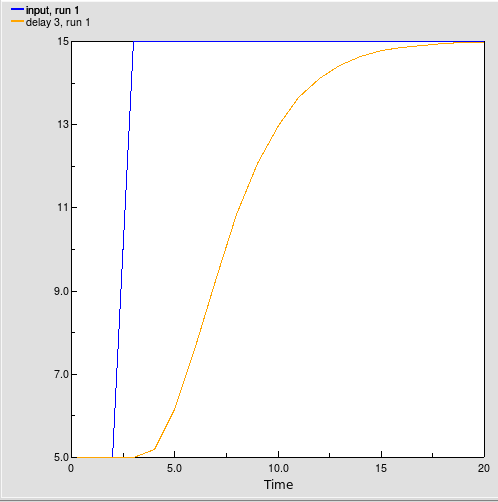
The delay1, delay3 ​and delayn function calculates a first, third or nth-order material delay of input, using an exponential delay time of delay duration, and an optional initial value initial for the delay. delay3 does this by setting up a cascade of three first-order material delays, each with a delay duration of delay duration/3. Other versions of the function behave analogously. delay3 returns the value of the final delay in the cascade. If you do not specify an initial value initial, all functions assume the value to be the initial value of input.

The delay3 function will return the value of delay 3 in the structure and equations shown in the following figure:

Compartment   comp1 : 
    Initial value = start_fill (real)
Compartment   comp2 : 
    Initial value = start_fill (real)
Compartment   comp3 : 
    Initial value = start_fill (real)
Flow   delay 1 : 
    delay 1 =         comp1*3/duration (1/day) 
Flow   delay 2 : 
    delay 2 =         comp2*3/duration (1/day) 
Flow   delay 3 : 
    delay 3 =         comp3*3/duration (1/day) 
Flow   inflow : 
    inflow =         input (1/day) 
Variable   start fill : 

    start fill =         initial*duration/3 (real) 

Example:

Delay 3 = delay3(input, 5) where input = 5 + step(10,3) produces the pattern shown below:


Built-in functions : first function

first function

first(T)

Takes an argument T that is a member of an enumerated type, and returns "true" if it is the first member of its type, and "false" otherwise.

Input: enumerated type member, or array of enumerated type members

Result: boolean, or array of boolean values

Examples:

If enumerated type "fruit" is defined as "apple", "grape", "banana":

first("apple") --> "true"


first(["banana", "apple", "banana"]) --> ["false", "true", "false"]

In: Contents >> Working with equations >> Functions >> Built-in functions

Built-in functions : following function


following function

following(T)

Takes an argument T that is a member of an enumerated type, and returns the next member of the enumerated type.

Input: enumerated type member, or array of enumerated type members

Result: enumerated type member, or array of enumerated type members

Examples:

If enumerated type "fruit" is defined as "apple", "grape", "banana":

following("apple") --> "grape"

following(["grape", "apple", "grape"]) --> ["banana", "grape", "banana"]

In: Contents >> Working with equations >> Functions >> Built-in functions

Built-in functions : forcst function

forcst(<input>,<time>,<horizon>[,<initial>])

New in v6.6

The forcst function performs simple trend extrapolation. Here's how it works. First, forcst calculates the trend in input, based upon the value of input, the first order exponential average of input, and the averaging time. (Think of the averaging time as the time over which you wish to calculate a trend.) Then forcst extrapolates the trend into the future - you specify the distance into the future by providing a value for horizon. If you do not specify initial, forcst substitutes 0 for the initial value of the trend in input.

The forcst function is equivalent to the structural diagram and equations shown in this figure:

Put diagram here

Compartment   Average input : 

    Initial value = input-(averaging*initial) (real)
Flow   change in average : 
    change in average =         (input-Average_input)/averaging (1/day) 
 Variable   averaging : 
    averaging =         Variable parameter (day) 
 Variable   forecast : 
    forecast =         input*(1+trend*horizon) (real) 
Variable   horizon : 
    horizon =         Variable parameter (day) 
 Variable   initial : 
    initial =         Variable parameter (real) 
Variable   input : 
    input =         Variable parameter (real) 
Variable   trend : 
    trend =         (input-Average_input)/(Average_input*averaging) (1/day) 

Example:

Sales_Forecast = FORCST(Sales,10,15,0) produces a forecast of sales 15 time units into the future. The forecast is based on current sales, and the trend in sales over the last 10 time units. The initial growth trend in sales is set to 0.

Built-in functions : in_preceding function

in_preceding function -- new in Simile v5.7

Usage: in_preceding(expression of any type) returns that type

Definition: Used in a multi-instance submodel, returns the value of the argument expression  as it would be in the preceding instance of that submodel, or 0 or "false" in the first instance. The argument can include the function prev(0) to refer to the value in the previous submodel instance of the component in whose equation the in_preceding() function appears.

Note that a model that contains a circular set of influences can build and run properly if the input parameter associated with one of the influences is only used in the argument of an in_preceding() function. This is because since the value of the argument is calculated for one submodel instance and then used in the next, there is no actual circular dependency.

Example 1:

A 5-instance submodel contains a variable with the equation

index(1)+in_preceding(prev(0)).

The values will be:

1 3 6 10 15

Example 2:

An 8-instance submodel contains two variables, "received" and "forwarded". These are connected to one another by influences in each direction. The equation for "forwarded" is received/2. The equation for "received" is

if index(1)==1 then 200 else in_preceding(forwarded)

The values of "received" for the 8 instances will be:

200 100 50 25 12.5 6.25 3.125 1.5625
In: Contents >> Working with equations >> Functions >> Built-in functions

Built-in functions : ramp function

ramp(time,slope)

Generates a ramp of slope slope, starting at time time and zero before that time.

Result: the ramp function.

Arguments: time at which to start ramping, slope (positive or negative) of ramp

Example:

the function ramp(20,-7) will have a return value of 0 at time 20 and -70 at time 30


Built-in functions : smth1, smth3, smthn functions

smth1, smth3, smthn functions

smth1(input, averaging [, initial])

smth3(input, averaging [, initial])

​smthn(input, averaging, n [, initial])

Arguments:

input: the value to be smoothed

averaging: time over which to smooth the input value

n (smthn only): order of the material smoothing

initial (optional): the value of the result when the function first applies

Result:

The smoothed value of input.

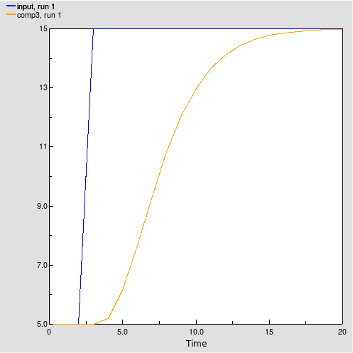
The smth1, smth3 and smthn functions perform a first-, third- and nth-order respectively exponential smooth of input, using an exponential averaging time of averaging, and an optional initial value initial for the smooth. smth3 does this by setting up a cascade of three first-order exponential smooths, each with an averaging time of averaging/3. The other functions behave analogously. They return the value of the final smooth in the cascade. If you do not specify an initial value initial, they assume the value to be the initial value of input.

The smth3 function will return the value of comp3 in the structure and equations shown below.

Compartment   comp1 : 
    Initial value = initial (real)


Compartment   comp2 : 
    Initial value = initial (real)

Compartment   comp3 : 
    Initial value = initial (real)


Flow   flow1 : 
    flow1 =         (input-comp1)*3/averaging (1/day) 

Flow   flow2 : 
    flow2 =         (comp1-comp2)*3/averaging (1/day) 

Flow   flow3 : 
    flow3 =         (comp2-comp3)*3/averaging (1/day) 

Examples:

Smooth_of_Step = smth3(Step_Input,5)

where

Step_Input = 5 + step(10,3) produces the pattern shown below.


Built-in functions : step function

step(height,time)

creates a step function. Output is 0 up until time, and equal to step thereafter.

Result: the step function.

Arguments: height of step, time at which to step.

Example:

step(30, 20) has output 0 at time 19, and 30 at time 20 and after

Built-in functions : stop function


stop function

stop(n)

Input: is a number (real or integer) of your choice

Result: None (see text)

When executed, this function halts execution of the model, and produces the following error message:

Simile ran into a problem trying to run this model.

While it was trying to calculate the value of variable

var (node x) during execution of the model at

time t, there was a user-defined interruption: n.

It is useful to define error conditions where you (the model designer) know that the model should not be used or is not applicable for some reason. Trivially, it can be used to guard against mathematical errors, for example:

if (time()-50) != 0 then 1/(time()-50) else stop(5)

This form has some merit when running in C++, but generally, to track down mathematical errors, it is easier to debug in Tcl. If execution in Tcl would take too long, then this is a useful alternative. Its primary use however, is to enable you to catch out-of-range conditions in the specific circumstances of your model.

The use of an error code in the user-defined interruption (e.g. stop(13) ) enables you to see which stop( ) function caused the model to stop running, if there is more than one in your model.

Result is undefined, because simulation stops at the point at which the function is called, but has integer type (this is important because if it is called in a conditional, the other branch of the conditional must also have a numerical type).

Examples:

if population>50 then stop(1) else 0

if (time()-50) != 0 then 1/(time()-50) else stop(5)

In: Contents >> Working with equations >> Functions >> Built-in functions

Built-in functions : trend function

trend(<input>,<time>[,<initial>])

New in v6.6

The trend function calculates the trend in input, based upon the value of input, the first order exponential average of input, and the exponential averaging time averaging time. trend is expressed as the fractional change in input per unit time. If you do not specify initial, trend substitutes the value 0 for the initial value of the trend.

The trend function is equivalent to the structural diagram and equations shown in this figure:

Put diagram here

Compartment   Average input : 

    Initial value = input-(averaging*initial) (real)
Flow   change in average : 
    change in average =         (input-Average_input)/averaging (1/day) 
 Variable   averaging : 
    averaging =         Variable parameter (day) 
Variable   initial : 
    initial =         Variable parameter (real) 
Variable   input : 
    input =         Variable parameter (real) 
Variable   trend : 
    trend =         (input-Average_input)/(Average_input*averaging) (1/day) 

Example:

Yearly_Change_in_GNP = TREND(GNP,1,.04)

This equation calculates the annual change in the input GNP. It starts with an initial value of .04 (4% per year).

Built-in functions : var_delay function

var_delay function

var_delay(var,n)

Input: a variable name and a numerical value (real or integer) of time units

Result: the value (any type) of the named variable, n time units ago

This function returns some previous value of another variable, an arbitrary period of time before. The period of time is defined in time units (not steps). The number need not be an integer, but whatever the actual time step, delay is always rounded to the nearest multiple of 0.1 of a time unit. The variable whose previous value is required is specified by name. The variables must be linked with an influence arrow.

This is a general replacement for the last( ) function, which returns the value of the named variable from the previous time step only. The delay must be between 0 and 100 and is rounded to the nearest 0.1. The delay can vary; if the delay is constant, the function const_delay() will do the job more efficiently.

Examples:

runoff=var_delay(rain,soak_time)

In: Contents >> Working with equations >> Functions >> Built-in functions

Built-in functions: at_init function

at_init function

at_init(X)

Returns the value the argument had when first used, i.e., on model reset or when the submodel instance containing this equation was created.

at_init(X) creates an implicit intermediate result, which has the same dimensions as its argument. So if this result is implicitly replicated elsewhere in the equation, the same value will be used each time. See makearray for behaviour in explicit replication.

Input: Any data type

Result: Same type as input

In: Contents >> Working with equations >> Functions >> Built-in functions

Built-in functions: at_posn function

at_posn function

at_posn(C)

at_posn(C,Row,Col)

Must form the whole equation of a component. Sets the component's value to the value of a component in an instance of a 2-D submodel representing a grid. C is the caption of the component in the grid submodel, and Row and Col if present are the outer and inner indices of the source instance (i.e., grid square) from which to get the value. If Row and Col are not present, the grid is mapped onto the diagram of the submodel containing the target component and the source instance selected by the component's position in the submodel diagram.

Input: Any data type plus optionally two integers

Result: Same type as input

In: Contents >> Working with equations >> Functions >> Built-in functions

Built-in functions: const_delay function


const_delay function

const_delay(var,n)

Input: a variable name and a numerical constant (real or integer) of time units

Result: the value (any type) of the named variable, n time units ago

This function returns some previous value of another variable, a arbitrary period of time before. The period of time is defined in time units (not steps). The number need not be an integer, but whatever the actual time step, delay is always rounded to the nearest multiple of 0.1 of a time unit. The variable whose previous value is required is specified by name. The variables must be linked with an influence arrow.

This is a general replacement for the last( ) function, which returns the value of the named variable from the previous time step only. The delay must be a numeric constant; for variable delay see var_delay().

Examples:

runoff=const_delay(rain,10)

In: Contents >> Working with equations >> Functions >> Built-in functions

Built-in functions: dies_of function


dies_of function

dies_of(X)

Returns true if argument is the loss channel that will cause the individual to disappear at the end of the current time step.

Input: value from a loss channel in the local submodel

Result: boolean

In: Contents >> Working with equations >> Functions >> Built-in functions

Built-in functions: in_progenitor function

in_progenitor function -- new in Simile v5.8

Usage: in_progenitor(expression of any type) returns that type

Definition: Used in a population submodel, returns the value of the argument expression  as it would be in the instance of that submodel containing the reproduction channel responsible for the instance being evaluated, or 0 or "false" in an instance that arrived via a channel other than reproduction. The argument can include the function prev(0) to refer to the value in the progenitor submodel instance of the component in whose equation the in_progenitor() function appears.

Note that a model that contains a circular set of influences can build and run properly if the input parameter associated with one of the influences is only used in the argument of an in_progenitor() function. This is because since the value of the argument is calculated for the progenitor instance and then used in the offspring instance, and the progenitor always comes before the offspring in evaluation order, there is no actual circular dependency.

Important: If the progenitor instance has been removed (see Extermination) then using this function will return meaningless values, and may cause model execution to be aborted due to memory access violations. To avoid this problem, make the in_progenitor function itself the argument of an at_init() function, e.g., at_init(in_progenitor(index(1))). If this is done, the inner argument will be evaluated for the progenitor instance when the offspring instance is created -- at which time the progenitor definitiely exists -- and then retained within the offspring instance's data structure. The only reason for not doing this would be if changes in the value in the progenitor continue to affect the offspring, and offspring never outlive their progenitors, e.g., in an L-systems model of tree branching.

In: Contents >> Working with equations >> Functions >> Built-in functions

Built-in functions: iterations function

iterations function

iterations(X)

Returns number of iterations that have been done up to this point in an alarm submodel. Argument is the boolean balue from the alarm symbol.

Input: value from an alarm symbol in the local submodel

Result: integer

In: Contents >> Working with equations >> Functions >> Built-in functions

Built-in functions: preceding function

preceding function

preceding(T)

Takes an argument T that is a member of an enumerated type, and returns the previous member of the enumerated type.

Input: enumerated type member, or array of enumerated type members

Result: enumerated type member, or array of enumerated type members

Examples:

If enumerated type "fruit" is defined as "apple", "grape", "banana":

preceding("grape") --> "apple"

preceding(["banana", "grape", "banana"]) --> ["grape", "apple", "grape"]

In: Contents >> Working with equations >> Functions >> Built-in functions

Built-in functions: pulse function

New in v6.6. Note this function is provided purely for compatibility with continuous-only modelling tools, and new models should use squirts instead.

pulse function:

pulse(magnitude, first_time [, interval])

Generate a pulse with a duration of a single time step and a given cumulative value.

Result: the pulse waveform

Arguments:

magnitude: the cumulative value of the pulse. This will be the level change of a compartment due to a flow with this value coming into it.

first_time: The first, last or only time at which the pulse will occur

interval (optional) : If this is positive, the pulse will occur regularly with this interval after the initial time

If it is negative, the pulse will occur with this interval up until the initial time and not after

If zero or not present, the pulse will occur only once at the initial time

Example: pulse(20, 12, 5) generates a pulse value of 20/DT at time 12, 17, 22, etc.


Built-in functions: trigger_magnitude function

trigger_magnitude function

trigger_magnitude()

Returns a value representing the magnitude of the triggering event. Can only be used in the equations of derived events, squirts and rule-based state variables. Events influencing these components are not listed as parameters so this function is used to get their values. If the trigger is a simple event, this function gives the value of that event's equation. If it is a time series, it is the current value from the series. If it is a limit event then it is 'true' if there is only one limit, and -1/1 for lower/upper limit if both are given.

Inputs: none

Result: same units and dimensions as triggering events


In: Contents >> Working with equations >> Functions >> Built-in functions

Built-in functions : sofar function


sofar function

sofar([X])

sofar({X})

Result is…

Input: numeric array/list

Result: numeric

Example:

Comment:

In: Contents >> Working with equations >> Functions >> Built-in functions

Built-in functions : size function


size function

size(S)

size(S,I)

The first form takes the name of a fixed-membership submodel and returns the number of instances that it has. The second form takes the name of a fixed-membership submodel and returns the size of the Ith level of nesting of this submodel.

Input: submodel name

Result: integer

In: Contents >> Working with equations >> Functions >> Built-in functions

Built-in functions : dt function


dt function

dt(I)

Returns the duration of the level I time step.

Input: numeric. This is the time step level.

Result: numeric

Examples:

dt(1) --> 0.1 (for a model whose top-level time step was set to 0.1 in the Run Control panel)

dt(2) --> 0.001 (for a model whose 2nd-level time step was set to 0.001 in the Run Control panel)

If you are starting off with Simile, it is unlikely you will need to understand the concept of "time step index". You will probably just be making models with a single time step, hence one level, so don't worry about anything except the use of dt(1).

The main use of the dt function is to engineer the addition or removal of a specified amount of a substance into or out of a compartment. The only handle we have for causing changes to the amount in a compartment are flows, and flows are expressed as a rate per unit of time (whatever time unit is used for the model, e.g. year). This creates a problem if we want to add or remove a specified amount of substance at some instant in time. For example, consider a model with a time unit of year, a time step of 0.1, and with a compartment X from which we want to remove 5 units at the instant that some condition, which only lasts for 1 time step (0.1 years), is met. If we simply had a flow out that was zero when the condition was not met, and was 5 when the condition was met, then for one time step the flow would be 5 (units per year): hence, only 0.5 units would be removed in the 1/10th of a year, not the 5 we intended. What we need to do is to artificially inflate the flow rate by a factor of 10 (in this case, with a time step of 0.1) for this one time step. We do this by dividing the flow rate (in our flow equation) by 0.1 (in this case), or by dt(1) in general. The flow rate then appears to be 50 units per year for that one time step, giving a loss of 5 units in the one time step. Bingo!

The actual flow expression for the case considered above would be:

flowout = 5/dt(1)

Special case

Using the argument zero in the function, i.e. dt(0), is equivalent to saying dt(n), where n is the time step index of the submodel in which the function is used. This is useful, because when a submodel time step index is changed, it is then not necessary to edit the dt() functions within it to preserve the meaning.

In: Contents >> Working with equations >> Functions >> Built-in functions

Built-in functions : count function


count function

count([X])

count({X})

Number of values in the array [X] or the list {X}

Input: array or list of values (numeric or boolean)

Result: integer

Examples:

count([4,5,6]) --> 3

In: Contents >> Working with equations >> Functions >> Built-in functions

Built-in functions : channel_is function

channel function

channel_is(X)

X is an immigration, reproduction or creation channel. Returns true if this individual appeared through that channel.

Input: numeric

Result: Boolean

Examples:

channel_is(cr1) --> true, for each instance of the population that was initially created through channel cr1.

Comments:

This function can only be used inside population submodels. Its argument is the name of a channel (i.e. a population control symbol, one of creation, immigration or reproduction). Note that the value of the channel itself is not used, just the name. The result can be used in calculations inside the population submodel. For example, the expression

land_owned = if channel_is(im1) then 0 elseif channel_is(cr1) then 10

would allocate 10 acres of land to each member of the original population, but none to immigrants.

In: Contents >> Working with equations >> Functions >> Built-in functions

Built-in functions : init_time function


init_time function

init_time(1)

Returns the time at which this model component first came into existence. This really only has any use for:

  • population submodels, so that the model knows when a new member of the population was created; and
  • conditional submodels, so that the model knows when the submodel, or one instance of it, came into existence because the condition controlling it became true.

Input: numeric. In fact, the argument is not used, so simply insert the number 1. The only reason for having the brackets and an argument enclosed between them is that this is the only way that Simile can recognise that this is a function.

Result: numeric

Example:

Let's assume you have a population submodel, and some property of each individual is related to its age (e.g. its growth rate, or its probability of dying). Simply create a variable called age (inside the submodel), and insert the following equation:

age = time(1) - init_time(1)

The result is the difference between the current simulation time (given by the function time(1), and the time when the instance was created, given by init_time(1).

In: Contents >> Working with equations >> Functions >> Built-in functions

Built-in functions : index function


index function

index(I)

Returns the index (instance number) of a member of a fixed membership or population submodel, for the level of submodel nesting specified by the argument.

Input: numeric

Result: numeric

Comment:

The index function is frequently used in conjunction with the element function when working with multiple-instance submodels: both fixed-membership and population submodels.

The argument specifies which index is to be returned. You can see summary information about the meanings of the different indices in the listbox headed Indices: in the equation dialogue. The argument is an integer between 1 and the maximum number of indices available. index(1) corresponds to the 'innermost' index, i.e., if you have one multiple-instance model inside another, the result of index(1) will be the index of the inner submodel instance, and the result of index(2) will be that of the outer submodel instance. Similarly, if a submodel has two dimensions, then index(1) and index(2) will be valid in that submodel, giving an instance's position along the inner and outer dimension respectively.

Relation submodels do not usually have indices of their own, but you can get the indices of their base submodel instances using the index() function. If one of the roles in a relation has been specified to 'allow base instance lookup', then the base submodel for this role will be 'innermost' and and the index of the instance in this role will be the result of calling 'index(1)' in the relation submodel.

For fixed-membership submodels, the function returns an integer value between 1 and n, where n is the number of instances for the submodel. For variable-membership submodels, it returns an integer between 1 and n, where n is the maximum possible index. For a population submodel this would be the total number of instances of the population that have ever existed during this simulation run. For a conditional submodel the maximum will be the size given in the submodel dimensions. For either of these, an instance with a particular index number may or may not exist.

In: Contents >> Working with equations >> Functions >> Built-in functions

Built-in functions : Statistics

Statistical functions produce variates from distributions, and generally produce different values at each point in the model where they are called.

There are up to three forms of each statistical function:

  • The form with a _const suffix. This will produce a new value when the simulation is initialized or reset, or when a submodel instance containing it is created. This value stays the same until the end of the run, or until the submodel instance containing it ceases to exist.
  • The form with a _var suffix (or no suffix). This will produce a new value on each time step for each instance where it occurs. The sequence of values for all such functions can be initialized using the Initialize pseudo-random tool. If there is no _const form of a function, the _const behaviour can be produced by wrapping this form in the at_init() function.
  • The form with an extra argument. The last argument (an integer) serves as a seed for the values produced by that particular occurrence of the function. These will be the same each run, and independent of any other statistical functions in the model. For instance if it is used in a conditional submodel, it will start producing the same sequence of results each time an instance of the submodel comes into existence (assuming the seed value is the same).

If a statistical function only has one form, it behaves like the 'var' form.

Built-in functions : rand_const function

rand_const function

rand_const(X,Y)

Returns a random number between X and Y at the start of the simulation or when the submodel instance is created. The random-number generator is not called again, and so the value stays the same until the simulation is reset.

Input: numeric, numeric

Result: numeric

Comment:

The main use of this function is to assign values to a set of instances of a multiple-instance submodel (fixed-membership or population). For example, to randomly assign initial sizes to a set of trees in a multiple-instance tree submodel, we could use the equation:

size = rand_const(12,20)

or to assign random locations to the trees, we could use the equations:

x = rand_const(0,50)

y = rand_const(0,100)

which would randomly place the trees in the left-hand half of a one-hectare plot, assuming that the values are in metres.

The use of rand_const() is deprecated because it cannot be made to behave in the same way as rand_var when implicitly replicating over an array. It is implemented by internal conversion to at_init(rand_var(x,y)) and this form should be used in full to make the replicatio behaviour clear.

Historical note: You may come across some models that use a rand(X,Y) function. This behaves like rand_const if Simile deduces that the model element will only be called at initialisation time, and like rand_var if the equation contains some variable that changes over time. The use of this function is now also deprecated because the semantics of the two uses are so very different. Also, there are some situations when you need to be able to over-ride this behind-the-scenes decision about how the function should behave.

In: Contents >> Working with equations >> Functions >> Built-in functions

Built-in functions : rand_var function

rand_var function

rand_var(X,Y)

Returns a random number between X and Y, with a new value every time step.

Input: numeric, numeric

Result: numeric

Comment:

This function is used for doing stochastic modelling and Monte-Carlo simulations, i.e. one or more processes in the model (like giving birth or dying) have a random element to them.

rand_var gives a new result for every call, and if it is used in an expression that is replicated to make an array, each element's random value will be different.

rand_var uses the pseudo-random sequence generator built into the c++ compiler which Simile is using to create executable models. The sequence is initialized with a value generated from the process ID and clock time when Simile starts up, so no two runs will produce the same results. However, if it is required that a model has exactly the same behaviour each time it runs, despite including calls to rand_var, this can be achieved by means of a tool that sets the seed to a given value; see Initializing pseudo-random sequence.

Historical note: You may come across some models that use a rand(X,Y) function. This behaves like rand_const if Simile deduces that the model element will only be called at initialisation time, and like rand_var if the equation contains some variable that changes over time. The use of this function is now deprecated because the semantics of the two uses are so very different. Also, there are some situations when you need to be able to over-ride this behind-the-scenes decision about how the function should behave.

In: Contents >> Working with equations >> Functions >> Built-in functions

Built-in functions : binome function

binome function

binome(prob, n)

Input: Real numerical value, integer value

Result: A value from the binomial distribution with the given probability and number of trials. A new random deviate is generated each time step.

The binomial distribution describes the probability of a given number of positive outcomes occurring when a number n of trials are carried out, each with a certain probability p of a positive outcome.

This function is implemented using a pseudo-random sequence generator; notes regarding its behaviour can be found in the documentation for the rand_var function.

Examples:

coins_heads_up = binome(0.5, coins_tossed)

In: Contents >> Working with equations >> Functions >> Built-in functions

Built-in functions : colin function

colin function

colin([Array])

Returns a deviate from a distribution whose relative probabilities are given by the values in the argument array. A new deviate is generated each time step.

Inputs: array of probabilities (real).

Outputs: index to value in array (int).

This can be used to make a deviate from an explicit set of probabilities where the pattern does not match any other built-in statistical function.

This function is implemented using a pseudo-random sequence generator; notes regarding its behaviour can be found in the documentation for the rand_var function.

Example:

colin([1,1,1,10,1]) --> 4 (usually), 1,2,3 or 5 (occasionally).

In: Contents >> Working with equations >> Functions >> Built-in functions

Built-in functions : exprnd function

exprnd function

exprnd(mean [, seed])

Returns: value sampled from an exponential distribution (numerical)

Arguments: mean of distribution (numerical), seed for random sequence (integer, only required if a reproducible series of values is needed)

Example: A Geiger counter pointed at a radioactive source will emit a series of clicks at random times. The durations of the intervals between the clicks are distributed exponentially.

In: Contents >> Working with equations >> Functions >> Built-in functions


Built-in functions : gaussian_var function

gaussian_var function

gaussian_var(mean, sd)

Input: Two real numerical values

Result: A random sample from a Gaussian (normal) distribution, with the supplied mean and standard deviation. A new random sample is generated each time step.

This function is implemented using a pseudo-random sequence generator; notes regarding its behaviour can be found in the documentation for the rand_var function.

Examples:

daily_rainfall = gaussian_var(annual_rainfall/365, 1.0)

In: Contents >> Working with equations >> Functions >> Built-in functions

Built-in functions : with_colin function

with_colin function

with_colin({ProbList},{ValList})

Takes two lists with equal size, and returns an element from the second argument, picked at random with the probability of each element proportional to the value of the corresponding element in the first argument. A new return value is generated each time step.

Inputs: list of probabilities (real), list of corresponding values (any).

Outputs: element picked from second list (any).

This can be used to make a deviate from an explicit set of probabilities where the pattern does not match any other built-in statistical function.

Note that it only works on lists; if you want to do something similar with fixed-size arrays, you can combine the element and colin functions to achieve the same effect as follows: element([ValList], colin([ProbList]))

This function is implemented using a pseudo-random sequence generator; notes regarding its behaviour can be found in the documentation for the rand_var function.

Example:

with_colin({1,1,1,10,1}, {"apples", "pears", "oranges", "grapes", "bananas"}) --> "grapes" (usually), "apples", "pears", "oranges" or "bananas" (occasionally)

In: Contents >> Working with equations >> Functions >> Built-in functions

Built-in functions: hypergeom function

hypergeom function

hypergeom(Pop, Mark, Sample)

Returns a deviate from a hypergeometric distribution for a given population, number of marks, and size of sample.

Inputs: Population size (int), number of marked individuals (int), size of sample from population (int)

Outputs: deviate of number of marked individuals from sample

The hypergeometric distribution tells us the range of probabilities of getting a number of "marked" individuals when taking a sample of a certain size from a population, a given number of which are "marked".

This function is implemented using a pseudo-random sequence generator; notes regarding its behaviour can be found in the documentation for the rand_var function.

Example: A research process involves ringing a certain number of seabirds from a population and releasing them, then at a later date recapturing a different number of the birds and checking how many ringed individuals are retreived. If a random group of individuals are captured each time, the probability of getting n rings back is equal to the probability of getting the result n from the equation:

rings_retrieved = hypergeom(Seabird_population, Birds_ringed, Birds_caught)

In: Contents >> Working with equations >> Functions >> Built-in functions

Buit-in functions : poidev function

poidev function

poidev(mean)

Input: Real numerical values

Result: A value from the Poisson distribution with the given mean. A new random deviate is generated each time step.

The poisson distribution describes the probability of a given number of positive outcomes occurring in the limiting case of the binomial distribution, i.e., with very many trials each with a very small chance of a positive outcome.

This function is implemented using a pseudo-random sequence generator; notes regarding its behaviour can be found in the documentation for the rand_var function.

Example: A hospital serves a large community in which a certain percentage of individuals are thought to be carriers of the hospital superbug MRSA. If we admit a small number of individuals to hospital, we would expect the probability of getting a certain number of MRSA carriers in that group to be equal to the probability of getting that number as the result of this equation:

MRSA_positive_admissions = poidev(Total_admissions*MRSA_prevalence_percent/100)

In: Contents >> Working with equations >> Functions >> Built-in functions

Working with equations : User-supplied functions

User-defined functions

There are three different mechanisms for users to supply functions for use in expressions:

  1. user-defined macros, which provide a short-hand for long or complex expressions that would otherwise have to be used repeatedly in expressions.
  2. user-defined external procedures, written in a programming language such as Tcl or C++.
  3. model-fragment function definitions (introduced in Simile v6), in which the behaviour of a function is implemented by a separate Simile model.

User-supplied function declarations and definitions should be put in files in the Functions directory in Simile's local data tree. This tree is created automatically when you first run Simile. Its location is:

  • On Windows: "My Simile Files", under "Documents" (Windows 7 or Vista) or "My Documents" (earlier Windows versions)
  • On Linux: .simile, in the user's home directory
  • On MacOS: Simile, in the user's home directory

Declarations and definitions in the Functions directory in Simile's installation tree (e.g., "Program files/Simile54") are for functions treated as "Built-In", i.e., expected to be available in any Simile system. It is worth looking at these for guidance in writing your own functions, as the formats are the same.

In: Contents >> Working with equations

User-defined functions : Macro definitions

Macro definitions

Macro definitions provide a shorthand for long, complex expressions that would otherwise have to be used in equations, possibly in several different elements. The definitions are stored in one or more external files, which are read each time Simile starts. Users may edit the files to include user-defined macros.

Each new macro is defined in a new line in any file with the extension .pl in the Functions directory. There are two places where this directory can be; one is within the Simile program files tree (for built-in functions), and the other is under Simile's local directory (for functions to be treated as user-defined). Any functions added by modellers should be placed in the latter location;  this has the effect that when a model requiring the functions is saved, they are marked as user-defined, and if the model is subsequently opened on a system where the function definitions are not present, a warning is displayed saying which user-defined functions are missing.

The format of the macro definition line is:

f(X1, X2 ... Xn) --> F(X1, X2 ... Xn).

where:

  • f is the name of the user-defined function. This has the format of a Prolog atom or variable, so it must start with a letter, and unlike the built-in function names it is case-sensitive.
  • X1, X2 … Xn are a series of one or more variable identifiers. These also have the format of Prolog atoms or variables, so they must start with letters and are case sensitive. These formal arguments to the function are replaced when the function is used, by the actual argument values. If the function requires no arguments, you must place a pair of single quotes between the empty parentheses.
  • F(X1, X2 … Xn) represents any expression that could be used in an element's equation. The variable identifiers can be used as quantities anywhere in this expression. This is the macro itself. As with any expression in the equation language, it may extend over more than one line.
  • The symbol '-->' means 'maps onto'. It, and the final period, are part of Prolog syntax.
  • Next line shows how to write 0-ary (no arguments) macro definitions (leave parentheses out) and macro definitions calling 0-ary functions or macros (put empty atom in parentheses).
    init_time --> at_init(time('')).
    Note the argument in the call is two single quotes, not a double quote.
     

The function, as it appears on the left side of the arrow, can then be used in any Simile equation, with any sub-expression taking the place of each of the variable identifiers. The result returned by the function will be the same as that which would have been returned by the expression on the right hand side, if the same sub-expressions had been substituted for the variable identifiers.

The .pl files distributed with Simile (and installed in the Functions directory in Simile's program files) contain a number of examples of function definitions. These include the following:

  • subtotals(Arr): Takes an array and returns another array of the same size containing the totals of all the values up to that point in the original array. e.g., subtotals([1,2,4,3]) = [1,3,7,10].
  • rankings(Arr) Takes an array and returns an array of integers of the same size each representing the position in the sequence of largest to smallest (largest = 1) of the corresponding value in the original array. e.g., rankings([8.2, -5.1, 2.5]) = [1,3,2].
  • with_greatest(Arr1, Arr2) Takes two arrays and returns the element of the second in the position corresponding to the largest-valued element of the first
  • colin(Arr) Takes an array and on each time step returns an integer, with the probability of each value being proportional to the value at that position in the original array.

Comment lines, starting with a %, can be included in this file, and standard multi-line comments bounded by /*...*/ can be used.

If there is a syntax error in a user function definition, this will cause a warning to be produced when Simile is started. The other definitions will still be usable.

In: Contents >> Working with equations >> User-defined functions

User-defined functions : External procedures

External procedural functions

To include user-defined external procedures, there are three files:

  1. A file under the Functions directory with the .pl extension. This file can also contain macro definitions. Procedurally defined functions that are treated as being built-in to Simile go in Simile's installation tree, while those that are treated as user-defined go in the local information tree. The declarations take one of two possible forms:

    function(Name, ResultType, ArgTypes).
    This form is used for ordinary, deterministic functions.
    sample(Name, ResultType, ArgTypes).
    This form is used for functions which give a new value each time they are called, even if the arguments do not change. This is used for stochastic functions such as gaussian_var, and is required because Simile otherwise tries to be lazy -- it only re-evaluates a function if the arguments change.

    In either form, "Name" is the name of the function, which is used in Simile's equation language. "ResultType" the type of the result - one of int, real, boolean or any - and "ArgTypes" a list of argument types in the same form. These allow the Prolog equation parser to accept this function in equations, and to put it into the target language program as a procedure call wherever it is used.

  1. procs.cpp -- This is in the same Functions directory as the function declaration. It contains the C++ implementation of the function. When the model is built in C++, during compilation of the generated code, this file is included (via support1.cpp) and linked into the resulting model library.
  1. procs.tcl -- contains the Tcl implementation of the function. This is sourced just prior to the model program, but not in global scope so any global variables used by the procedure need to be declared both inside it and out.

These files are stored in the Functions directory of the Simile program files tree. If you wish to build models in both C++ and Tcl, using the same function name, you must include the function definition is both procs.cpp and procs.tcl.

It is generally not a good idea to use global variables in the function definitions, because if the functions are used in more than one place in the model, a value set when running one instance of it may be used when running another instance.

In: Contents >> Working with equations >> User-defined functions

User-defined functions : Model Fragments

Model Fragments as Function Definitions

This feature, introduced in Simile v6, is really, really easy to use. Suppose you need to have a particular function available in your model, and you have no idea how to program it in c++ or write a macro expression for it, but you can easily make a simple Simile model that implements the function. One option would be to build such a model, and copy it to every part of the model you are working on where you need the function it provides. The trouble is, this would make the diagram confusing and the model would be harder to maintain, since if you changed the implementation of the function you would have to change all the occurrences of the model fragment that carries it out.

Now you can keep the model fragment somewhere else, and refer to it wherever you like by means of an ordinary function. The fragment goes in a directory called Fragments which is a subdirectory of either of the Functions directories for user-defined functions in general. The name of the function it implements, and the components of the fragment which correspond to the result and arguments, are identified by the name of the fragment file, which has the format 

functor,result,arg,... .sml

For instance, suppose you want a function that returns the first prime number greater than its argument. You could make a model fragment that looks like this:

Model fragment implementing 'next prime number' function

This model takes a number in the 'start' variable, and generates the next prime number up from it in the 'next' variable. It uses two nested iterative submodels. The outer one tries each odd number, starting from 'start', until one is found to be prime. The inner one applies the test for primeness, dividing the candidate by each odd number starting from 3 until either an exact factor is found, or the next divisor is greater than the square root of the candidate. If a factor is found, the outer submodel moves on to the next candidate and the inner one starts again.

So, we have our model, how do we make the function? By saving it in the Fragments directory with a name made of the following parts:

  • The name of the function, in this case 'next_prime'
  • The caption of the model component that has the result, in this case 'next'
  • the captions of all the arguments in the order in which they will appear in the function call, in this case just the one: 'start'

These are all separated by commas and the name finishes with the .sml extension as for any Simile model, so the full name is

next_prime,next,start.sml

Now you can use the function in any equation, e.g. "next_prime(z)>50"

Points to note:

  • The argument components must be variable parameters as shown above.
  • The result and argument components must be in the top level of the model fragment, i.e., not in a submodel
  • ​The fragment can include compartments, in which case the function will have a state and its output will depend on its inputs at earlier times
  • If you use an array as an argument to a function where it is a single value in the definition, you will get a separate instance of the fragment for each element of the array
  • The internal components of the fragments will appear in the model explorer during execution and their values can be inspected
  • Fragments can include any Simile feature, including functions defined by other fragments (but avoid circular definitions!)

In: Contents >> Working with equations >> User-defined functions

Working with equations : Graph function

Graph function

The Sketch Graph window is called from the equation dialogue when the modeller wishes to sketch, by hand, the relationship between two variables. The relationship is, mathematically, a function: that is, there is only one Y value possible for any given X value.

The graph is sketched using the mouse. The graph consists of a number of straight-line segments. The x-coordinates of the two ends of each segment is fixed, but the y-coordinate of each end can be dragged up or down with the mouse. The y-coordinate at the end of one segment is constrained to be the same as the y-coordinate at the start of the next, making a continuous, if angular, curve. The modeller can vary the number of line segments used to make up the curve: if this number is quite high, then a close approximation to a smooth curve can be obtained.

The function is actually evaluated using linear interpolation. On any one occasion, there will be a single value for the x (independent) variable. The function calculates which line segment this occurs in, and how far along the line segment it lies. Simple algebra is then used to calculate the corresponding value for the resulting dependent (y) variable. Alternatively, you can choose to have the exact y value for the closest defined x value to the one given; see "options" below.

The window itself does not show the names of the variables involved. The independent (X-axis) variable is not yet specified at this stage, since that only happens when the user returns to the Equation window. The x value can be any Simile expression. There does not need to be a specific variable associated with y-axis, since the result of evaluating the graph function is just like any other function result - a value to be incorporated into the rest of a mathematical expression: graph(weight) plays the same role in an equation as log(weight), for example.

Click the OK button to return to the equation dialogue window. New text reading "graph()" has been inserted into the expression field, if this is the first time the sketch graph has been used for this equation. You must insert, between the brackets, the name of the independent (x-axis) variable or other expression. If you have already entered a graph() expression in the equation dialogue box, then the opportunity is given to edit the previously-drawn curve. It is not possible to use two different graph() functions in the same expression.

Drawing the curve

The curve is constructed by moving the mouse into the graph pad, holding the mouse button down, then moving the mouse from left to right (or from right to left) along the desired path. You are unlikely to get it right first time. If a line segment ends up in the wrong place, just try again. For finer control, you can click on a vertical line at the required point: the ends of the two line segments meeting at this line will then jump into position.

Scaling the axes

The two edit fields along each axis (Min and Max) are used to indicate the range of each axis. You click in the edit field, then enter a value that is appropriate to the lower and upper limits respectively of the variable in the relationship. Thus, if the independent variable were temperature, and we were modelling a site in Africa, then the x-axis might be scaled to be between 10 and 40 (the units of degrees Celsius are implicit). When you change the scaling of an axis, the actual sketch stays the same, so the behaviour of the function is changed to correspond to the new axis scaling.

By default, "Min" and "Max" are 0 and 100 respectively on both axes. It is not permissible to leave any entry blank.

Current position

These two edit fields display the current position of the mouse pointer in the graph area whilst dragging the curve. You can use this display to exercise finer control over the curve. It is also possible to enter values directly into these boxes, copying values from a table for example. After entering the Y-value, press the return or enter key on the keyboard to have the graph re-drawn to include the new pair of values.

If you want exact values for all the points in the graph, click the "Edit as table" button, and enter them with the keyboard, or by cutting and pasting.

Options

Between points

The normal behaviour of the graph function is to interpolate between the two nearest defined y values to get the function's result. Alternatively you can select 'Round' here, in which case you get the exact y value for the nearest defined argument value. The shape of the sketch graph changes to illustrate the actual values returned.

Out of range

There are three options to determine what happens if the independent variable falls outside the range scaled in this window, whilst the model is running.

  • truncate: this option extends the curve horizontally to the left and to the right.
  • extrapolate: this option extends the curve along a line with the same slope as the first and the last segment.
  • wraparound: this option joins up the left and the right ends of the curve. It is useful for defining repeating functions like sin(x).

X axis resolution

Clicking on the right-arrow button doubles the number of vertical lines in the graph pad area; clicking on the left-arrow button halves the number of lines. The higher the resolution, the greater the number of line segments making up the curve, and the smoother the curve is.

Altering function while model is running

The behaviour of the sketch can be altered while the model is running, using the edit sketch helper. This does not affect the version of the function in the saved model.

In: Contents >> Working with equations

Working with equations : Table function

Table function

The table dialogue window is used to create a table from data stored in a file. The required data are extracted from the file, and saved with the model. The table function is appropriate when referring to a relatively small amount of data which will always be the same wherever the model is used, for instance, the number of days in each month of the year. If you do not wish or need to store the data in the model, you can use a file parameter to access the data when the model is run. This is significantly quicker; so much so, that for extremely large data sets it is the only feasible approach.

There are three main uses of the table function:

  • entering a value for some variable for each instance of a multiple-instance submodel;

  • entering time-series data; and

  • entering a relationship between two variables.

In all cases, the table dialogue window is accessed through the equation dialogue window of a variable. Each variable can store one table. Because it is implemented as a function, the table can be used in the equation for the variable together with other components. Each table has one or more indices, which are used to extract a particular item of data from the table.

For example, a series of samples of soil quality might have two indices, an x- and a y-coordinate. The data value would record the soil quality for each (x,y) pair. The table function would then be table(x,y) and would return the value representing soil quality at the given coordinates. In this case, x and y could be influences from other variables or could be derived from the index of a multiple-instance submodel. In other cases, the index might be derived from simulation time.

Loading the table data

When you hit the 'Table...' button, the table data dialogue appears. This is the same dialogue that is used to load the data for a file parameter, and is used in the same way. Therefore, your data can be in any of the formats that are supported for file parameters -- but remember that very large datasets will be handled inefficiently, so use file parameters instead. The data is stored as an array in the model, so any indices loaded from the file must be integers.

Using the table function

The table function always takes at least one argument, and if there is more than one index, takes as many arguments as there are indices. It returns the item of data referred to by the arguments. Each application of the table function makes use of a different source of its arguments. We now examine these in turn.

Entering a value for each instance of a multiple-instance submodel

Suppose that we have a model that contains multiple instances of some type of object: for example, multiple patches of land, multiple trees in a stand of trees, or multiple species of vegetation in an area. We have a file containing actual data for this scenario: for example, a database containing elevation and slope data for the patches of land; species, height and diameter for the trees; or growth rates and initial biomass for the vegetation.

Create the table, selecting as data column the column containing the data you wish to use. Do not specify an index. The row number will be used instead. Return to the equation dialogue window by clicking OK.

Notice that Simile has automatically inserted table() into the Equation box. Change this to table(index(1)) : this indicates that each value in the column of data from the file will be assigned to the corresponding instance number in the model.

Entering time-series data

Many ecological models include exogenous variables, such as temperature or rainfall, which influence the behaviour of the model but are not themselves influenced by it. Sometimes the modeller is content to generate values inside the model, using a time-series generator to produce a sequence of values with appropriate statistical properties. Often, however, historical records exist, and the modeller wants to use these in the model.

As stated above, the table() function is only appropriate if the amount of data is relatively small and it is to be stored as part of the model. If you have large datasets which you want to load into the model as it runs from a separate file, you should look at working with time series data.

The quickest way to include a small time series in your model is to have a data file, as specified above, with at least two columns: one for the variable of interest (e.g. temperature), and one giving the time when each temperature measurement was made. Drag the column heading corresponding to the variable of interest (say, temperature) into the Use as data column edit box. Drag the column heading corresponding to the simulation time into the list box labelled Use as indices.

The text table() is inserted into the equation box. Change this to table(int(time())). Because time() returns a floating point number, the int() function is used to convert it to an integer. The text now reads table(int(time())).

There is more information on working with time series in the Working with External Data section of the help.

Entering a relationship between two variables

In this case, one or more other elements are used as the argument(s) to the table function. For example, if we have a series of pairs of temperature and rainfall values that produce different growth rates, we can use the expression table(temperature, rainfall). Note that both arguments must be integers. If they are not, use the int() function to convert them.

In: Contents >> Working with equations