Getting started: how to build and run a simple model
Getting started: how to build and run a simple model
This section takes you through the whole process of building and running a model as quickly as possible. The exercise is based on a simple model of a bank account, since we are all familiar with this context, and we can readily do the calculations ourselves. This should save you from thinking that there is something mysterious about how Simile calculates the behaviour of a model.
The model: a simple bank account model
Step 1: Starting Simile: what's on the screen
Step 2: Making the model diagram
Step 3: Adding initial values, parameter values and equations
Step 4: Initialising the model
Step 5: Choosing the output displays
Simple bank account model
The model: a simple bank account
We will make a model for a simple bank account, with interest paid annually at a rate of 10%, and $10 taken out every year. The account initially contains $300. This is what we expect to happen:
Year 1
|
Opening balance |
$300.00 |
|||
|
Interest paid in |
$30.00 |
0.1 x 300 |
||
| Withdrawal |
$10.00 |
|||
|
Closing balance |
$320.00 |
300 + 30 - 10 |
Year 2
|
Opening balance |
$320.00 |
|||
|
Interest paid in |
$32.00 |
0.1 x 320 |
||
| Withdrawal |
$10.00 |
|||
|
Closing balance |
$342.00 |
320 + 32 - 10 |
Year 3
|
Opening balance |
$342.00 |
|||
|
Interest paid in |
$34.20 |
0.1 x 342 |
||
| Withdrawal |
$10.00 |
|||
|
Closing balance |
$366.20 |
342 + 34.2 - 10 |
And so on. Note that the increments are getting bigger each year because each time the balance goes up, so the interest paid increases. The balance of the bank account is increasing at a faster and faster rate.
Having understood the calculations that we are going to perform, we now turn to the concepts needed to express these ideas in Simile.
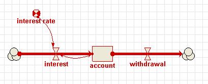
We use a compartment to represent the amount of money held in the bank account, since this a quantity that changes incrementally over time. We use two flows, one to represent the gain of money from interest and the other to represent the loss of money by withdrawal. One flow (interest) will go into the compartment, while the other flow (withdrawal) will come out of the compartment. We will also use a variable to represent the interest rate (10%, or 0.1). This variable will be linked to the flow representing the payment of interest by an influence arrow, indicating that the amount of interest paid depends on the interest rate. Since the amount of interest paid also depends on the amount in the bank account, there we will also use an influence arrow from the compartment representing the bank account to this flow.
In this tutorial we want to introduce you mainly to the mechanics of working with Simile, and these are explained in detail in the following steps. The concepts involved in representing even a simple system like this one in a modelling language can be quite complex.
Step 1: Starting Simile: what's on the screen
Step 1: Starting Simile: what's on the screen
Starting Simile
 You start Simile by double-clicking on the desktop icon created during installation, or by clicking on the Simile icon in the Start Menu.
These are both shortcuts to the file <Simile Program Files>\System\bin\Simile.exe, where <Simile Program Files> is the directory you chose to install the program. By default, this is commonly "C:\Program Files\Simile50", though if you are using a network, it may be on a remote hard drive. If you would like to be able to start Simile from a different location, create a shortcut to this file.
Linux users can start Simile by typing the command 'simile' in a terminal. Also, a shortcut is added to the Science/Education submenu of the Applications menu, which can be dragged to the desktop or taskbar, depending on your desktop environment.
On a Mac, Simile will be added to the Applications folder, from which it can be dragged to the desktop or task bar.
Within a few seconds, the main window will be displayed.
The Main Window
When Simile starts, you see a single window. This contains:
- a menu bar (at the top of the screen on a Mac), containing a standard File menu, some menus specific to Simile, and a Help menu. Hold the mouse over the title for each menu to see the options it contains.
- a toolbar, extending over two rows. The top row has standard tools (e.g. for opening and closing files), plus some specific to Simile.
- a component bar, containing buttons corresponding to each type of model-diagram element: you will use these for building up your model diagram. The right-hand part contains buttons for editing the model diagram. Hold the mouse over each button to get a brief description of its function.
- an equation bar, for entering equations into the model. At the right-hand end of the equation bar are the tools to accept or reject changes to equations, and to help build equations.
- a big blank area (the "desktop canvas") with faint lines. This is where you will draw your model diagram. The grid can help you arrange your diagram neatly.
Step 2: Making the model diagram
Step 2: Making the model diagram
We begin by drawing the model diagram for the bank account model. A note on colours used in the following description: when you add a component to the model diagram, it is initially drawn in blue. This means that the component is selected. You will see the ways in which this is useful later on. When the component is not selected, it will turn red. This is its usual colour, and means that the component needs some extra information (like a value or equation) before the model can be built.
1. Add a compartment to the model diagram.
- Click on the
 compartment symbol in the toolbar.
 - Move the mouse to the middle of the desktop window, and click again.
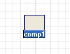
You should see a box labelled comp1.
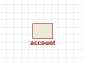
2. Rename the compartment "account".
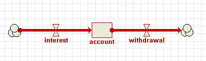
3. Add an interest flow and a withdrawal flow.
- Click on the
 flow symbol in the toolbar.
 - Move the mouse into some space to the left of the compartment labelled account, hold the mouse button down, and drag the mouse into the centre of the compartment. Release the mouse button.
- Type in the label interest.
- Move the mouse into the centre of the compartment, and drag to the blank area to its right. Release the mouse button.
- Type in the label withdrawal.
As an alternative to dragging out the flow, you can just click on its start and finish positions.
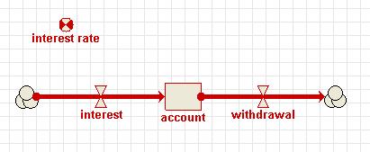
4. Add a variable for the interest rate
- Click on the
 variable symbol in the toolbar.
 - Move the mouse to the blank area above the interest flow, and click once.
- Type in the label interest rate.
7. Draw the influences
- Click on the
 influence arrow button in the toolbar.
 - Move the mouse to the middle of the compartment labelled account, and drag an influence arrow to the flow labelled interest.
- Release the mouse button when the flow has turned green.
- Move the mouse to the middle of the variable labelled interest rate, and again drag an influence arrow to the flow labelled interest.
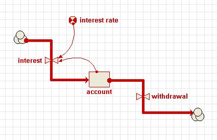
8. Re-arrange the model diagram
- Click on the
 pointer button in the toolbar.
 - Move the mouse to the middle of the compartment labelled account.
- Drag the mouse, and watch the compartment and its associated arrows re-arrange themselves.
- You can also move the following components:
- the cloud symbol at the end of each flow arrow;
- the variable;
- the valve symbols on the flows;
- the middle of an influence arrow;
- the position of the "kink" that appears in a flow arrow when it goes between two components that are not exactly above, below or to the left or right of one another; and
- the labels. (A note on moving captions: if a component is selected, and is coloured blue, then the caption can be edited. To edit a caption, click on the label and type. You can drag the mouse to select a range of characters. To move the label relative to its component, make sure the component is not selected. You can then drag the label into its new position.)
This completes the drawing of the model diagram. In the next step, you will provide the numeric values and equations you need for simulating the behaviour of the bank account. Note, however, that this sequence (complete the model diagram before providing any quantitative information) is followed here for convenience: in general, you are free to provide the quantitative information at any stage in the diagramming process.
Step 3: Adding initial values, parameter values and
Step 3: Adding initial values, parameter values and equations
1. Prepare to set component properties
 pointer button in the toolbar.
2. Assign the initial value for the compartment
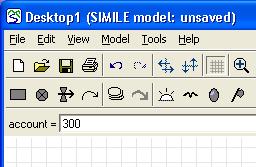
- Click on the compartment labelled account.
- Enter the value 300 into the equation bar.
- Click on the
 green tick mark or press the Return key.
3. Add the interest rate equation
- Click on the flow labelled interest.
- Variables account and interest_rate are now listed as influences upon interest. These influences are visible by clicking on the xs button. Selecting an influence from the drop-down list, places the text in the equation bar.
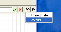
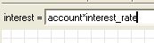
- Enter the expression account*interest_rate into the equation bar, either by selecting each variable in turn or by typing. Be sure to use an underscore rather than a space in interest_rate.
- Click on the green tick mark.
4. Assign the value for the withdrawal flow
- Click on the withdrawal flow.
- Enter the value 10 in the equation bar.
- Click on the green tick mark.
5. Assign the value for interest rate
- Click on the variable labelled interest rate.
- Enter the value 0.1 in the equation bar.
- Click on the green tick mark.
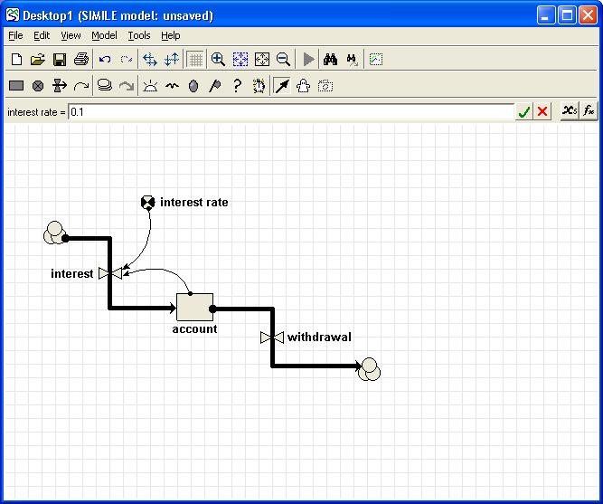
Notice that every component of the model diagram is now black, rather than red as it was before. This indicates that every component has been mathematically specified, and so the model is ready for running: Simile has enough information to work out the flows, and thus to update the amount of money in your bank account forward through time.
Step 4: Preparing to run the model
Step 4: Preparing to run the model
This and subsequent steps assume that you are using the single-window Run-Time Environment. This is the default, so it is the one that you will be using if you have installed Simile and not changed your Preference settings. If the windows that appear when you come to run the model differ from the ones shown here, then please go to the "Edit" menu, select the "Preferences" item, and then select the "Use single-window Run-Time Environment" option.
1. Run the model
- Open the Model menu
- Select the Run item.

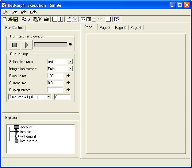
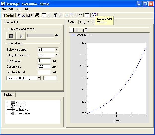
Simile creates a new window: the execution window. This contains the controls for running the model; a list of the variables in the model; and an area where any of a variety of tools for showing model results can be displayed.
2. Change the time step
Simile supplies a default time step of 0.1 when you first run a model. In natural science, a time step shorter than the time unit results in greater mathematical accuracy, but here we are dealing with an unnatural example; a bank paying compound interest on the balance of the account at the start of each year.
The above screenshot was taken from Simile v4; in v5 and later, the run settings are displayed on a separate tab within the run control notebook. Click on this tab to get at them, and then on the Run Control tab again to get the main controls back.
- Change the value for Time step #1 from 0.1 to 1.
This is because we want to use a time step of 1 year rather than the default value of 0.1 years.
3. Change the duration of the simulation run
- Change the value for Execute for from 100 to 10.
This is because we want to run the model for just 10 years at a time.
Step 5: Choosing the output displays
Step 5: Choosing the output displays
1. Select the graph-plot display
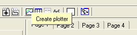
- Click on the
 "Plotter" display tool on the toolbar; or select it from the list in the Add menu.
2. Choose the variable you wish to have displayed
Note the graph window that appears. This is initially scaled with default values on both axes, but will rescale itself as needed. You can re-size the panel containing the graph by dragging on the little boxes on the horizontal and vertical panel separators.
- Click on the
 "Add a variable" button on the plotter toolbar
 - Click on the compartment labelled account in the list of model variables.

You can either click on the line representing the compartment in the "Explorer" tab at the bottom left of the execution window, or you can go back to the model diagram and click on the compartment there.
Step 6: Running the model
Step 6: Running the model
1. Start the simulation
-
 Click on the "Play" button in the Run control dialogue window.
Note the line that appears on the graph.
2. Continue the simulation
-
Click on the "Play" button again.
The simulation carries on for another 10 years.
Step 7: Repeating the model edit/run cycle
Step 7: Repeating the model edit / run cycle
1. Return to the desktop canvas
- Click on the "Go to Model Window" toolbar button.
2. Prepare to edit the component properties
- Click on the
 pointer button in the toolbar.
3. Change the interest rate from 10% to 15%
- Click on the interest rate variable.
- Change its value from 0.1 to 0.15
- Click on the green tick mark.
4. Run the model again
 Click on the "Run" button on the toolbar.
The model will automatically rebuild, re-initialise and run again.
Step 8: Saving and loading the model
Step 8: Saving and loading the model
1. Save the model to file
- Select the "Save As…" item in the File menu in the main (model diagram) window.
- Navigate through the file directory system in the normal way, to the directory where you wish to save the model.
- Enter a name for your model, and save it.
2. Loading a model from file
Either:
- Select the
 "Open…" item in the File menu
 - Search for your model.
- Click on the OK button.
or:
- Select the "Reopen -->" item in the File menu
- Select from the list of recently-used models