Working with submodels : Interfacing a network model with a grid

Interfacing a network model with a grid

If you have a modelling problem in which you are dealing with reservoirs of a substance at different locations, with varying transfers to and from them, you would normally choose one of:

• a single instance model with a network of compartments and flows representing reservoirs and transfers
• a multi-instance model disaggregated into grid squares, with a compartment representing levels in each square, and transfers between them making use of an association

Each of these approaches has its strengths, but in some situations we may wish to combine the two. For instance, we may be modelling a hydrological problem in which water diffuses through a region as groundwater, but which also contains reservoirs from which water is taken for industrial or agricultural use. Because we are interested in water dynamics over the entire area we would use a grid model, with a neighbour association to handle diffusion between adjacent squares, but we would also want to include associations between squares at larger distances to represent water transport by engineering such as pipelines and aqueducts. It would be possible to build a grid submodel with separate relations for neighbours and longer connections, but representing the water supply network as an actual network in its own submodel makes the model easier to understand and maintain.

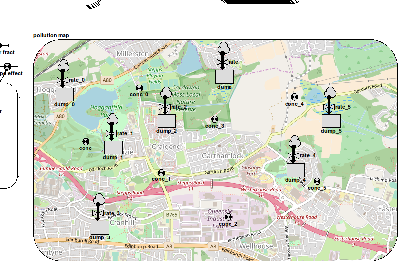
Simile's system for integrating models like this takes its inspiration from the ModFlow/WEAP interface, a system for connecting a network model in a special-purpose water engineering tool with a grid-based hydrology model. As in WEAP, the compartments in the network model are laid out within their submodel boundary according to the actual position of their corresponding features in the landscape being modelled. Thus the submodel appears like a topographical map of the water features on the landscape. To make the location of the features clearly readable, an actual map of the region can be used as a background image in the submodel, such as is shown in the image at the top of this page.In order for a component in the network model to get its value from the right instance of the corresponding component in the grid model, you would normally use the element() function with three arguments -- the parameter name associated with the grid component, and the row and column indices of the instance. This would be messy, requiring influences to each network component as well as working out and entering the actual indices. So instead we provide the at_posn() function, which as its name suggests, gets the value of the grid component in the instance at the corresponding position. Its only argument is the grid component's caption, and it must be the whole equation. An alternative form has three arguments, adding the row and column indices which replace those derived from the component's position. This is for use in cases where it is impractical to use the component's position in its submodel to select the grid instance, as in the case where a lot of them occupy a small region of the grid. The network model components now behave similarly to ghosts of the referenced component instances for the appropriate grid squares.

Any component can use the at_posn() function as its equation, provided it has the same quantization (discrete vs continuous) as the corresponding grid component.  For instance, in the diagram at the top of this page, the variables captioned conc_n all have the equation at_posn(concentration) and can be used to plot a graph of the pollutant concentrations at their positions on the map.

The network model can thus get values from the grid, but if the component is a compartment, its value will not be affected by transports (flows/squirts) in/out of the rest of the network model. These transports must now be directed to/from the grid instance compartment, and this currently requires some extra bits and pieces to be added to the model by hand. Suppose you have a grid model representing the diffusion of a pollutant around a watershed. That model might contain a compartment called 'pollutant' representing the amount of it in each square, along with flows carrying it between neighbouring squares according to concentration and transport rate. Now, if we want to show pollutant being added at various points on a separate map-related submodel, we would add compartments to it at the appropriate positions with flows going in representing rates of addition, and equations set to at_posn(pollutant). To get these to affect the grid submodel, we add a further submodel called 'pollutant_flows'. This gets three variables, 'stock_x', 'stock_y' and 'transp'.

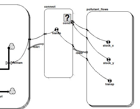
These names are recognized by Simile when the model is built, and the submodel properties are automatically edited to make it a multi-instance submodel with an instance for each flow connected to a compartment whose equation is at_posn(pollutant). 'stock_y' gets the row indices in the grid containing 'pollutant' for the positions of these compartments, either from their actual locations in their submodel or from the 2nd argument of at_posn() if present, while 'stock_x' similarly gets the column indices. 'transp' gets the values of the flows themselves (negated if they go out of the compartment concerned). The modeller may do anything she wants with these values, but the intention is to use them to set up a flow to the compartment in the grid submodel. This is most simply done by creating an association submodel between the grid and the submodel picking up the flow values (called 'connect' in the diagram). Here, 'transp' and the new flow 'contam' have the values 'role2_transp' and sum({'transp_role1'}) respectively, to simply pass the values between instances according to the relation. 'role1' has 'Allow base instance
lookup'  selected in order to use one-sided relation enumeration to set up the relationship as efficiently as possible, not that this matters with only a handful of flows, and to do this the equation for cond1 must be 'index(2) is role2_stock_y and index(1) is role2_stock_x'

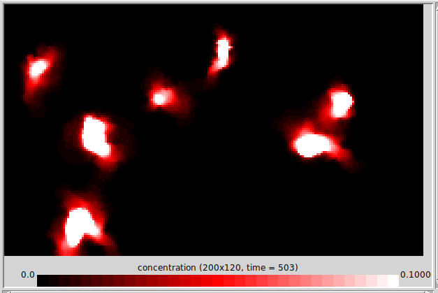
 There will now be an instance of 'connect' relating each flow in the network model to the grid model instance where it takes effect. This image shows the grid helper displaying pollution hotspots resulting from the flows in the first image (note the correspondance between the positions of the pollution hotspots and the positions of the compartments within the map submodel in that image).

If your network model has squirts instead of, or as well as, flows that must affect the grid model, you should add another specially-named submodel to handle them, and interface that to the grid submodel as described above. The differences are as follows:

• its name should be target_squirts rather than target_flows (target is 'pollutant' in the example)
• the 'transp' component inside it is a derived event rather than a variable, which will occur when the corresponding squirt does
• the derived event in the relation model and the squirt in the grid model have the equation 'trigger_magnitude()'
• The influences connecting them have their properties set up so as only to include source events corresponding to the roles of the relation.

In: Contents >> Working with submodels