Here’s an example of a model with two simultaneous equations implemented in Simile. It is a version of the Ball-Berry stomatal conductance model where assimilation (photosynthesis) is a function of stomatal conductance and stomatal conductance is a function of assimilation.
Where there is a big change in stomatal conductance (Gs) more iterations are needed to reach a certain accuracy.
The iteration submodel is at time step #2. This and its contained submodels have a time step of 0.01 in the run control. The rest of the model has a time step of 1. The iteration thus runs 100 times for each time step of the container submodel.
Equations in Desktop
Equations in Assimilation
Variable A : Assimation (umol CO2 m^-2 s^-1)
A = A_Q*last(Gs_0)
Where:
Gs_0=../Gs
Variable A_Q : Assimilation light response curve
A_Q = graph(Q)
Where:
Q=../../../Environment/Q
Comments:
Relationship of Assimilation with photon flux density (light) when stomatal conductance (Gs) is maximum
Equations in Environment
Variable C_a : Carbon dioxide concentration (umol CO2 (mol air)^-1)
C_a = graph(time())
Comments:
Typical diurnal curve in forest canopy
Variable H : Relative humidity (proportion)
H = graph(time())
Comments:
Typical diurnal graph (24 hour)
Variable Q : Photon flux density (umol m^-2 s^-1)
Q = graph(time())
Comments:
Graph for a sunny day (24 hours)
Equations in Iteration
Variable Gs : Stomatal conductance (mol m^-2 s^-1)
Gs = if time()==time then Gs else g_0+g_1*A*H/C_a
Where:
A=Assimilation/A
time=../time
H=../../Environment/H
C_a=../../Environment/C_a
g_0=../g_0
g_1=../g_1
Gs=../Gs
Comments:
Ball-Berry equation
Variable errorGs
errorGs = Gs_0-last(Gs_0)
Where:
Gs_0=Gs
Equations in Ball-Berry
Variable A
A = A
Where:
A=Iteration/Assimilation/A
Variable Gs
Gs = if time()==0 then g_0 else last(Gs_0)
Where:
Gs_0=Iteration/Gs
Variable errorGs
errorGs = last(errorGs_0)
Where:
errorGs_0=Iteration/errorGs
Variable g_0 : Stomatal conductance in the dark (mol m^-2 s^-1)
g_0 = 0.01
Variable g_1 : Ball-Berry stomatal conductance coefficient
g_1 = 23
Variable time
time = time()
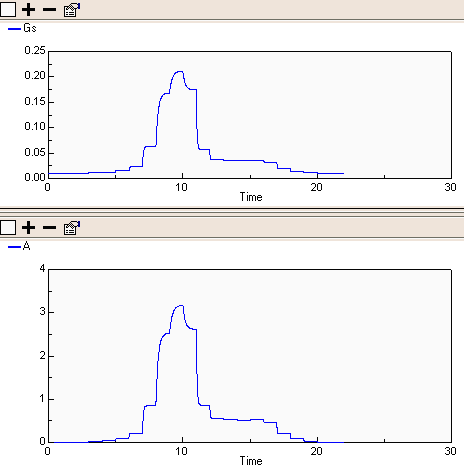
This first pair of graphs shows the calculated Stomatal Conductance and Assimilation on an hour-by-hour basis throughout the day.

This second pair shows the internal model representation of the two variables converging on the required hourly value. Note that when the magnitude of changes in the variables is large, as it is around time()==10 units, the convergence takes longer.

J. T. Ball, I. E. Woodrow, J. A. Berry. 1987. A model predicting stomatal conductance and its contribution to the control of photosynthesis under different environmental conditions. In: Progress in Photosynthesis Research, ed. J. Biggins. M. Nijhoff Publishers, Dordrecht. Vol. 4, pp 221-224.
- Vincent P. Gutschick : Regularities in Plant Control of Evapotranspiration and Carbon Gain Across Sites: Tests with Scaling Up and Modelling Consequences for Water and Carbon Balances
| Attachment | Size |
|---|---|
| 122.82 KB | |
| 12.72 KB |
