Worked example Simile models
These example models are provided to illustrate different aspects of modelling. All the models are quite simple, but will hopefully provide some inspiration in the creation of your own models. In addition, three models are saved in the “Examples” subfolder of the Simile program files directory. Also in this folder are the helper configuration files needed to visualise model behaviour.
|
Environmental and Ecological Science |
|
|
Sample food chain |
|
|
Five different approaches to modelling population dynamics |
|
|
Spatial model of de-forestation |
|
|
Life Science |
|
|
Modified Hodgkin-Huxley equations for neural membrane action potential. |
|
|
Utilities |
|
|
Submodel for calculating statistics descriptive of given input data |
|
|
Submodel for interpolating between irregularly spaced data points |
|
|
Fun |
|
|
Lorenz mathematical model of air turbulence. This model illustrates strange attractors and chaotic wandering. |
|
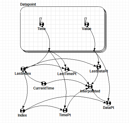
Datapoint interpolation
This is a submodel that calculates an interpolated value for a function defined by a fixed, irregularly spaced set of data points. It does simple linear interpolation, extrapoilating the line between the last two datapoints at either end to cover the domain outside the spread of datapoints. The descriptions are oriented to its use to calculate interpolated values from a time series, but the independent variable called CurrentTime could actually be any argument for the interpolated function.
Include this in your model, and make sure the submodel 'Datapoint' is set to the same number of instances as you have time points in your file.
Load the two fixed parameters with the data from your columns of time points and values respectively. Hint: if you do not drag any headings into the indices table, it will use the row number as the index. The rest of the model segment works out the interpolated value for the current time by finding the indices of the last and next time points and scaling the values at those times.
Download the model file and include it in your own models using Simile’s plug-and-play features.

| Files : |
| Attachment | Size |
|---|---|
| 18.6 KB |
Descriptive statistics
This is a submodel that calculates statistics describing the distribution of values of a single variable stored in an array. TestDescriptiveStats.sml includes the DescriptiveStats submodel that can be used in your own models by using plug and play. It could also be extended to calculate further statistics.
The following statistics are calculated:
- Mean
- Variance
- Standard deviation
- Average deviation
- Kurtosis
- Skewness
Two test data sets are provided :
|
File |
Mean |
Standard deviation |
|
params11.spf |
1.0 |
1.0 |
|
params12.spf |
1.0 |
10.0 |
These test data are from reference data sets produced by the EUROMETROS (a European Collaboration in Measurement Standards project) for evaluating the numerical accuracy of the results produced by scientific software.
These data are not time series and so there is no need to run this model, since the calculations are done instantaneously. Running for a longer period will cause exactly the same calculations to be repeated each time step. Of course, if the input data were varying, as they would be in your own model, then the descriptive statistics will change each time step to reflect the changing data.
Example to calculate the statistics for the data in params11.spf:
- Open the model in Simile
- Run the model.
- When the "Enter file parameters" dialog appears click the "Load File" button and choose params11.spf
- Examine the values of the variables by mousing over the variables on the model window or model explorer or load the display configuration file TestDesriptiveStats.shf to have the values displayed in a table.
Download the model file and include it in your own models using Simile’s plug-and-play features.
| Files : | DescriptiveStatistics.zip |
Ecosystem energy flow
This model represents the flow of energy through the different components of an ecosystem. It is a classic compartmental model, conforming to conventional System Dynamics notation, and could be represented in any of the standard System Dynamics visual modelling packages.
The model has five compartments, representing the energy content (in joules perhaps) in each of five ecosystem compartments:
- the primary food chain, consisting of
- plants
- herbivores
- carnivores
- the detritus chain, consisting of
- detritus
- detritivores
The flows show the processes that move energy from one compartment to the next. The overlapping circles represent clouds, signifying a System Dynamics ‘source/sink’: in effect, a compartment outside the system, whose value we are not interested in. The thin arrows represent influences, and indicate which compartments are deemed to influence each flow: i.e the flow rate is dependent on the value in the compartment.
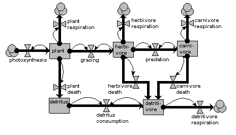
Note that, though very simple, there are still significant design decisions indicated here. For example, the feeding flows are shown to be dependent on the amounts in both the food compartment and in the feeding compartment. Also, we assume here that dead plant material goes into a detritus compartment, because of its relatively long residence time, whereas dead animal material is consumed immediately by the detritivores.
Hodgkin-Huxley equations
This model was created by Dr. John Fowler, of Texas Tech University Health Sciences Center, and implements the Hodgkin-Huxley equations describing currents across a neuronal membrane that contribute to the action potential. Hodgkin and Huxley published this model in 1952 and received the Nobel Prize in Physiology/Medicine, in part for this work, in 1963. Dr. Fowler has added an additional conductance from work by Connor and Stevens, 1971.
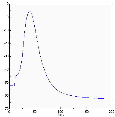
This graph shows a simulated action potential triggered by an injection of current at t=10 msec. Using the model, the underlying currents can also be graphed to determine their contribution to the action potential.
Download the model file and explore its behaviour, perhaps using Simile’s plotter, which is set-up by the included display configuration file.
| Files : |
We are grateful to John C. Fowler, PhD, Physiology Department, Texas Tech University Health Sciences Center for permission to distribute this model. Please contact Dr. Fowler with any comments on the model.
Land-use change
The model illustrates three types of submodel and is an example of a spatial model implemented in Simile. It shows that Simile is capable of handling quite complex spatial behaviour — in this case, landuse change in which the neighbours of a patch influence the likelihood of transition from one landuse state to another — even though Simile has no built-in constructs for spatial modelling.
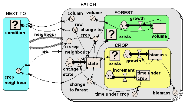
The model illustrates three types of submodel:
- The PATCH submodel is a fixed-membership, multiple-instance submodel, and is used to represent the fact that there are many landuse patches. Each patch has row and column attributes, and each one is engineered to have a unique combination of values between 1 and 20, thereby defining each one’s position on a grid. (But to drive home the point: Simile understands nothing from the labels “row” and “column”: it is up to us, the modellers, to ensure that these are given values which can be used as grid co-ordinates.)
- The FOREST and CROP submodels are contained inside the PATCH submodel. Therefore, each patch can (potentially) contain both a forest and a crop submodel. However, note that each one is a conditional submodel: see the question-mark “condition” symbol in the top-left of each one, and note the little rows of dots leading from the bottom-right edges. This indicates that the submodel may exist in only some of the patches, not all of them. In fact, the conditions are engineered so that each patch contains only forest or crop, not both (but it would be quite possible for us to have some agroforestry patches containing both, if that’s what we wanted.)
- Finally, the NEXT TO submodel is an association submodel, defining an association (relationship) between some patches and others. We can see that this is an association between patches by the presence of the two broad grey arrows (role1 and role2), pointing from the PATCH submodel to the NEXT TO submodel. As the name suggests, this association defines which patches are next to which other patches. Again, it has a condition symbol, which is used to indicate under which conditions the association holds. We note that this has influences coming from the row and column variables in the PATCH submodel: the condition is true when the row and/or column value for one patch is one away from the row and/or column value of another patch.
The model works as follows. Each patch contains a state variable (the compartment “state”) which defines the state it starts off in. This is 1 for forest and 2 for crop. If a crop patch has been a crop patch for a certain length of time, then it is abandoned and reverts to forest (as mediated by the variable “change to forest”). If the volume of the trees exceeds a certain amount and the patch has crop neighbours (this is why we need to know which patches are next to which others), then the forest is cleared and it changes to crop as the landuse (as mediated by the variable “change to crop”).
The following figure show how the model behaves, using Simile’s grid map display to show the patches on a spatial basis. The light (yellow) squares represent the patches under crop; the dark (green) squares represent forest. When users request this display, they are required to specify a variable indicating the column number for each patch, and the actual variable to be displayed: Simile then has sufficient information to lay the patches out in the correct grid-based manner. This display shows how Simile can handle spatially-referenced information, even though it has no built-in concept of spatial modelling.

Initially, most of the area is forest, with a band of cropping land on the left. After 40 years, patches of forest on the forest margin have been cleared, leading to a ragged edge to the forest boundary. In this particular run, the model was set up so that there was no reversion of cropped land back to forest, but as indicated above it has been designed to allow for this to happen.
Download the model file from the model catalogue entry to see how the spatially-explicit model is formulated.
Lorenz strange attractors
In 1963 the meteorologist and mathematician E. N. Lorenz published solutions for a simplified mathematical model of atmospheric turbulence in an air cell under a thunderhead. The model is now generally known as an illustration for chaotic behaviour and strange attractors.
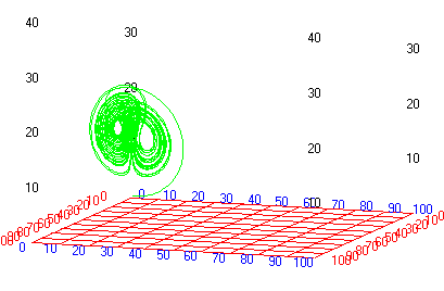
The basic equations are:
|
d(x1)/dt = a*(x2-x1) |
|
d(x2)/dt = (r-x3)*x1-x2 |
|
d(x3)/dt = x1*x2-b*x3 |
where:
- x1 is the amplitude of the convective air currents
- x2 is the temperature difference between the rising and falling currents
- x3 is the deviation of temperature from the mean
- a, r and b are dimensionless physical parameters
For more information, see http://mathworld.wolfram.com/LorenzAttractor.html.
Download the model file and explore the behaviour of the strange attractor using Simile’s included XY-plotter, as set-up by this display configuration file.
| Files : | lorenz.zip |
Population dynamics
The following sequence of five models illustrates two things. First, it shows that one problem — that of modelling changing population size — can be approached in a variety of ways, based on quite different methods for representing the population. Second, it introduces you to a range of constructs that Simile provides for modelling, including the “population submodel”, array variables, and the “association submodel”.
1. A lumped population
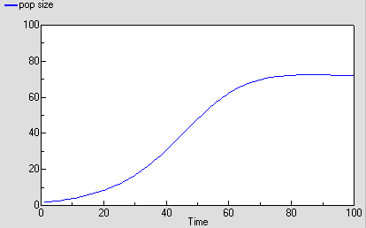
In this model, the population is represented by a single compartment, representing the total number of animals in the population or the population density (number per unit area). Reproduction is assumed to be density dependent (the reproductive rate per individual, r, declines as population size increases), whereas mortality is not (the mortality rate per individual, m, is independent of population size).
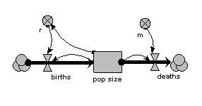
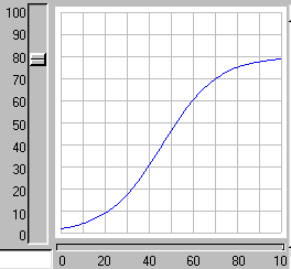
When the model is run, it shows the expected logistic form of population growth. When there are 80 individuals in the population, the birth rate balances the death rate.
2. Age classes, with a separate compartment for each age class
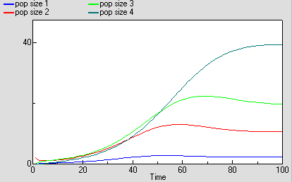
The same population is now represented by four compartments, one for each of four age classes. The first one represents the first year group, the second represents the number of animals aged 1-5 inclusive, the next animals aged 6-15 inclusive, and the fourth for all remaining animals. As before, the mortality rate per animal is independent of population size, but now depends on its age (there is a different m value for each age class). The reproductive rate per individual is still influenced by total population size, as well as now being different for each age class. Note that the first age class does not reproduce, so we simply do not include its reproductive rate.
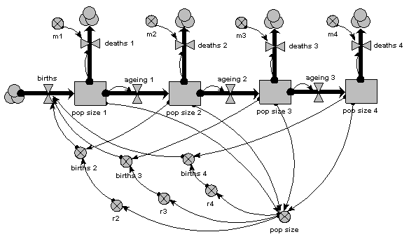
As before, we can now run the model and plot the dynamics of the total population size: this is in the variable called “pop size”, which is simply the sum of the population sizes for each age class. This again shows logistic growth: it will differ in detail, since the single-valued parameters we had before are now different for each age class.
But we are now able to inspect the dynamics for each of the four age classes. We see that the stable total population size is reflected in stable numbers in each of the four age classes, with different numbers in each class reflecting their different population parameters. Notice that there is some overshoot before the stable values are reached.
3. Age classes, with a multiple-instance submodel
The above two examples are expressed in conventional System Dynamics terms. They set the scene for the next three, which are now expressed in terms unique to Simile.
The second example had just four age-classes, but already we can start to see some problems. First, the diagram is starting to get a bit messy: this would get worse if, for example, the mortality rates were also density-dependent. Second, any change to one of the basic equations, such as that for working out the birth rate per individual, has to be done separately for each age class. We can easily see that this approach does not really scale up to a larger number of classes: for example, if we decided to have one-year classes for the whole population. What we would like to have is a way of specifying once how an age-class works, then get this repeated automatically across all age classes.
In other visual modelling environments, this is done by allowing the user to specify that some variables are in fact arrays. In Simile, the approach is to specify the compartment-flow structure in a submodel for one age-class in terms of scalar (single-valued) variables, then specify that the submodel has multiple instances, one for each age class.
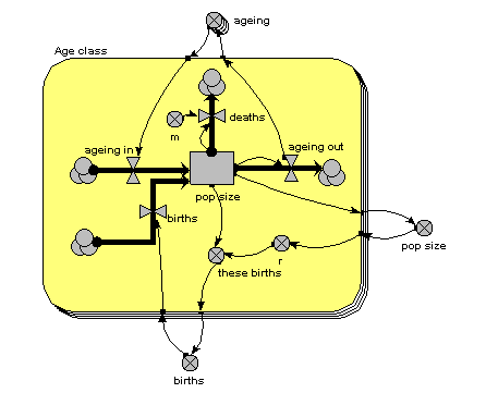
The main thing to note about this diagram is that it now has just one compartment. This is in a multiple-instance submodel, called “Age class”, with four instances, one for each class. The variable “pop size” inside the age class submodel represents the population of each age class; the variable with the name “pop size” outside the submodel represents the total population size (and is the sum of the population sizes for each age class).
What previously was a single ageing flow connecting two successive compartments is now two flows: one for the number leaving a compartment through ageing (“ageing out”), the other for the number entering a compartment from the class below (“ageing in”).
How does the “ageing in” flow for one age class know what the “ageing out” flow is for the class below it? This is clearly central to the whole model: everything else can be done on a class-by-class basis, but this involves some form of connection between classes. And we can't do that inside the submodel, since each instance can only know about its own values, not those of other instances. The answer is to take the “ageing out” values outside the submodel, and put them into an array (“ageing”). This array is them made available to the “ageing in” flow, which extracts the value for the previous class.
There is a births inflow for each age class. This is required since we are modelling a generic age class, but in fact the equation for this flow sets it to zero for all classes except the first. This flow is derived from the total births, which is held in the variable outside the age class submodel: that in turn is calculated from the sum of “these births”, which is the number of births for each of the age classes. Remember in the previous model how the first age class did not reproduce, so we simply left off the variables for it? We can’t do that now: instead, we set the parameter value r to zero for the first class.
The behaviour of this model is identical to the previous version, in which we had a separate compartment for each age class. We have not changed it mathematically: merely the way it has been implemented.
4. Age classes, using a multiple-instance submodel and an association model
The previous method is a big improvement: it is a much more concise way of representing multiple age classes, and exactly the same model can be used regardless of the number of classes we have: in other words, it scales up to larger problems. However, it suffers from a couple of disadvantages:
- There is a problem with the amount of data flowing around. Let’s say that we have 100 classes. Then Simile has to handle 100x100 values, since it has to make the array holding the 100 values available to each of the 100 classes. This is actually manageable, but still involves a lot of unnecessary computation (when we consider that in fact that there are only 100-1 = 99 interactions between classes, one for each pair of ageing transitions).
- Our model diagram does not really convey the fact that there is a special relationship between classes, namely that one class is immediately above the previous one. Class 2 is above class1, class 3 is above class 2, and so on. There is no connection between class 1 and class 3. Since this is an important feature of our model, and since one aim of the model diagram is to convey information about the model design down to a certain level, it would be nice if the model diagram showed that some form of relationship existed between classes.
Simile’s association submodel provides a way for tackling both problems. This is quite a big step in your understanding of Simile if you have not come across it before, particularly if you have no background in relational databases or the concept of “association” in object-oriented software engineering. So all I will do here is to present the model diagram and talk you through that: an explanation of the equations used can wait until you actually come to use it.
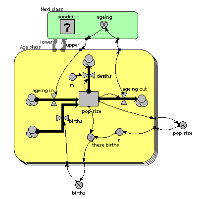
The only difference from the previous model is that the single array variable, holding all the ageing flows from one age class to the next, has been replaced by am ageing variable inside another little submodel, called “Next class”. This is made with Simile’s submodel tool, just like any other submodel. It is, however, different in two respects from other submodels. First, it has two broad grey arrows pointing to it from the “Age class” submodel. These indicate that there is an “next class” relationship (or “association”) between one class (the lower one) and another (the upper one). Second, we see that the submodel contains a condition element: this is used to specify the condition under which the “next class” relationship holds true. In fact, it holds true if, and only if, the instance number of one class is just one higher than that of another class: that condition is entered in the Equation box for the questionmark symbol.
What happens is that all the values for “ageing out” are passed to the submodel, but only one value is passed back into the submodel for each class: the one for the class above it.
You will have noticed that the model diagram does not itself tell us just what relationship exists between classes. However, it does tell us that some sort of relationship exists between them, so the diagram has helped in communicating the nature of the model down to a certain level. This is rather like when we have a variable with influences on it: we can see that the influences exist, without seeing the actual equation used to capture their effect.
5. Using a population submodel
The above examples all share one thing in common: they represent a population in terms of the values for one or more state variables, there being as many state variables as there are classes in the population. Each state variable may be engineered to have integer values (on the basis that populations contain a discrete number of individuals), or to have real (floating point) values, if you are content to think in terms of population density (i.e. number per unit area) rather than absolute numbers. The number of state variables (hence the computational requirement) is fixed, and totally independent of the number of individuals in the population.
A totally different approach is to represent each individual in the population separately. This can be justified on the basis of what is considered necessary to adequately capture the factors driving population dynamics. For example, if we know that social interactions between individuals is important, then we need some way of capturing these: it may be difficult to approximate to their effects in a lumped or class-disaggregated model.
Since we are interested in population dynamics, building an individual-base model will require that we create new individuals as time goes on, and remove existing ones. Thus, the amount of memory required to manage this population will change as the simulation proceeds. If the model is implemented by programming, the difficulty of doing this increases substantially as we move from a fixed number of state variables to a dynamically-changing list.
In Simile, it is very easy to create an individual-based model. You simply use a Simile submodel to define how one individual works, then declare this submodel to be a population submodel. You can then add model elements to hold the equations or rules for the creation of new individuals and the killing off of existing ones.
Here’s a model which is the individual-based equivalent of the age-class model with density-dependent reproduction. We make a submodel and call it “Individual” (following the principle that the label for a multiple-instance submodel should reflect the single object it references). It is specified as a population submodel by simply choosing this option in the submodel properties box. A population submodel is drawn with shadow lines on the top-left and bottom-right, to distinguish it from the fixed-membership multiple instance submodel we have seen so far.
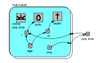
It has symbols for representing the initial number (i.e the number created when the model is initialised), an expression for creating new individuals by reproduction of existing ones (“birth”), and an expression for deciding when an individual dies (“death”). For consistency with the notation of the earlier models, we have two parameters, r and m, with similar meaning as before: r represents the probability that an individual will reproduce in one unit of time, and m represents the probability that an individual will die. Both r and m depend on the individual’s age (calculated simply as the difference between the current simulation time and the time when the individual was created). r also depends on the size of the population (negative density dependence). The population size is calculated as the sum of the value 1 (held in the variable “one”) over all the individuals. Note that population size has to be outside the individual submodel, since it is an attribute of the whole population, not of any one individual.
This model is now a stochastic one: the parameters r and m are treated as probabilities rather than deterministically generating changes to the population. We could have handled these deterministically - for example, creating one new individual when we had accumulated sufficient credit — but a stochastic interpretation is more intuitive. We could also have made the previous models stochastic (by sampling from a distribution to get the annual reproductive inputs and mortality losses), but then we would have lost the link with standard textbook models of population dynamics.
You may be surprised to see that there are no compartments here. We could have them: for example, we may want to model the change in body weight of each individual (or, say, height of each tree), in which case we could have a compartment and associated flows inside the submodel. We could equally well choose to have a complex System Dynamics model if, for example, we have a sophisticated, physiologically-based model of tree growth and we want to model a stand of trees on that basis. But this example shows that we do not have to include compartments and flows in a Simile model. Nevertheless, we can still use part of System Dynamics notation: the variable and the influence arrow.
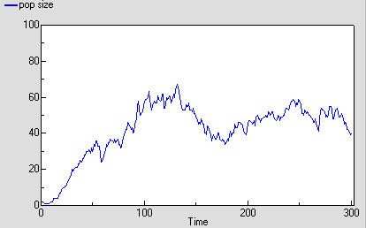
The following graph shows one run with the model. It’s run for 300 time units, since the reaching of an asymptote after 100 time units is less clearcut with this stochastic model. Even then, its stochastic nature means that there is considerable variation after reaching balance.
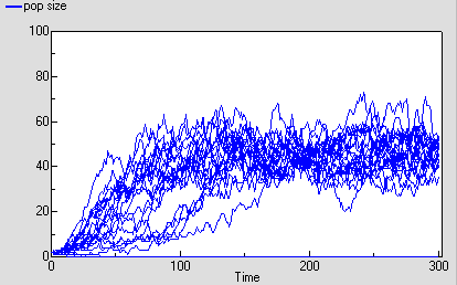
The following diagram shows the result for 25 replicate runs. The basic logistic growth can be discerned. It is also clear that the stochastic nature is more than simply variation around this line: some runs take quite a while to take off, and in fact in some cases the population goes extinct.
6. Conclusions
These five examples have demonstrated a number of important points.
- First, the population modeller can construct very different models based on more-or-less the same biological assumptions. The above models all have negative density-dependence for reproduction and density-independent mortality, but differ in their degree of disaggregation and the age-dependency of population processes. The modeller should be aware of these choices, and ideally be able to justify a choice vis-a-vis the alternatives.
- Second, mathematically-identical models (the three age-class models) can be implemented in different ways. These do not affect the results produced, but do affect the ease of working with the model and the ease of communicating the model to others. Again, the modeller should be aware of such choices.
- Third, Simile is unusual — if not unique — in enabling these very different models to be constructed within a single, easy-to-use environment. This minimises the amount of effort the modellers have to put in to explore these alternative approaches, compared with having to use different packages, or implementing the different models in a programming language.
Finally, we can broaden our vision beyond the modelling of one population. Usually, a population model will be a component of some larger system: the food on which the population depends; other predator populations; various abiotic factors; possibly even human factors (for example, in farming systems or wildlife conservation). Any of the population models we have considered above could be integrated into a larger, ecosystem model. Moreover, it could be wrapped up in an outer submodel envelope, and the alternative versions could be swapped in and out of the ecosystem model on a plug-and-play basis: another strong argument for enabling different modelling approaches to be implemented within a single modelling environment.