
Main menu
You are here
Built-in functions : fmod function
fmod(X,Y)
Returns remainder after dividing X by Y
Inputs: numeric, numeric
Result: numeric
Examples:
fmod(7,3) --> 0.333 (7/2 = 2.333, i.e. the remainder is 0.333)
fmod(time(1),1) --> a result that climbs from 0 to 1 repeatedly (i.e. a sawtooth pattern) as the simulation proceeds. See comments below.
fmod((index(1)-1),5)+1 --> 1,2,3,4,5,1,2,3,4,5,1,2,3... for successive values of index(1). See comments below.
This apparently obscure function in fact has (at least) two very valuable uses.
First, it can be used to generate regular cycles, in particular annual or daily cycles. Consider the case or a model with the time unit being one year, and a time step of less than a year. You want various exogenous variables (such as temperature or rainfall) to vary in a prescribed fashion during the course of each year, with the annual pattern repeating itself from one year to the next. The following diagram is typical of the model fragment you could use for representing this:
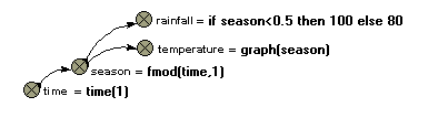
The variable time is simply set equal to current simulation time, using the function time(1). The variable season is set to rise from 0 to 1 every year. If your model used a time unit of one week, then the equation would be changed to
season = fmod(time,52)
and the value for season would then correspond to week number. The equations for rainfall and temperature are for illustration purposes only: you would need to replace them by something appropriate.
Second, the fmod function can be used to generate a regular spatial arrangement (rows and columns) for a 2D grid. Let's say that you are modelling an area of 10x10 grid squares. In Simile, you would set up a submodel, called perhaps Patch, with 25 instances. In order to give each patch location on a grid, each one needs to have a row and column attributes, with each patch having a unique combination of the numbers 1..5 for row and column. The only thing we know about each patch is that it has an index number (given by the built-in function index(1)), a value ranging between 1 and 25. The trick is to get row number to be, in sequence,
1,1,1,1,1,2,2,2,2,2,3,3,3...
and column number to be, in sequence,
1,2,3,4,5,1,2,3,4,5,1,2,3...
thus giving each of the 25 instances a unique row-and-column pair.
This is readily done using the following two equations:
row = floor((index(1)-1)/5)+1
column = fmod((index(1)-1),5)+1
See the floor function to understand why the row numbers should be in the first sequence above. For column, we divide the index number for each instance by 5, taking the remainder: the '-1' and +1' are there to ensure that we get the results in the blocks of five that we require. See a grid-based spatial model example to see this in action.
In: Contents >> Working with equations >> Functions >> Built-in functions
- Printer-friendly version
- Log in or register to post comments