Main menu
You are here
Population dynamics: single species: chaotic
This version differs from the standard population model in two respects:
- the growth rate depends on the current population by a quadratic relation. This will cause the population to approach the point of zero growth; and
- we consider time as being discrete rather than continuous. Rather than using a very small time increment between model states it is set equal to the time unit.
The behaviour of this model approximates that of a population where new individuals arrive all at once at a certain time of year, and most deaths also occur within a short period each year.
X(t+1) = g X(t) (1 - X(t)/100)
where:
X(t) = population size (number of individuals, or number of individuals per unit area) at time t g = growth rate (number of new individuals for each existing one with no resource constraints)

Compartment level
Initial value = rand_const(50,50.000001)
Rate of change = + change
Flow change
change = gain*level*(1-level/100)
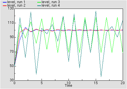
This graph shows the results of four consecutive runs with gain set to 1.4, 1.9, 2.3 and 2.7 respectively. On the first two runs the level approaches equilibrium; on the third it oscillates around the equilibrium, and on the final run it shows chaotic behaviour. Other behaviours such as period doubling will be shown for other values of gain.

This graph illustrates the unpredictability of chaotic behaviour. The model includes a very small random variation in the initial value of level, but the values for three consecutive runs, all with gain set to 2.7, diverge after about 60 time units. Until this time, the plot for the last run (green) exactly overwrites the other two.
